When I have to tell people what I work on, one of the phrases that I like to use is “physics-inspired sampling”. It does a good job conveying the gestalt situation: I’m a Physics PhD student who now works in statistics and machine learning.

But a lot of people are understandably confused about why a Physics PhD student would be working in statistics.

“Statistics? Like what sports fans use to win arguments on the Internet? What does that have to do with physics?”

It’s a decent question: what does statistics have to do with quantum mechanics? Or gravity? People with STEM backgrounds might be aware of some applications of statistical physics in machine learning—maybe not in detail, but in a vague “my freshman roommate from undergrad who now works at Google does stuff like that” kind of way.

But it turns out the connection between sampling and physics is quite old. Dating back to the middle of the 20th century, many sampling algorithms were either outright invented by physicists or invented to help solve some physical problem.

The Monte Carlo method was invented by the physicist Stanislaw Ulam (in collaboration with John von Neumann) during the Manhattan Project. It was developed to aid with the required nuclear-physics calculations.
The Metropolis algorithm was also invented at Los Alamos by a group of physicists (including Edward Teller, father of the hydrogen bomb) shortly after World War II.
Simulated annealing was proposed in 1983 by Kirkpatrick, Gelatt, and Vecchi, drawing directly on the metallurgical process of annealing—heating a material and slowly cooling it to reach a low-energy crystalline state.
Langevin dynamics adapts the equation Paul Langevin wrote down in 1908 to describe a particle jittering in a fluid (Brownian motion) into a recipe for sampling from an arbitrary distribution.
Hamiltonian Monte Carlo was invented by a team of physicists to help with lattice quantum chromodynamics calculations.
Diffusion models, one of the most powerful generative-modeling techniques in modern machine learning, were introduced by a team of Stanford physicists drawing on principles from non-equilibrium thermodynamics.

It’s pretty remarkable how persistent the connection between physics and sampling has been. From the Metropolis algorithm to diffusion models, physicists keep finding that the mathematical machinery they developed to describe nature also provides the right tools for drawing samples from probability distributions.

This makes a certain kind of sense. Physics is, in large part, the study of how systems explore their state spaces over time. Sampling is, in large part, the study of how algorithms explore probability distributions over time. That these two problems share so much mathematical structure is not an accident—it reflects something deep about the relationship between dynamics, randomness, and probability.

Markov-Chain Monte Carlo

Monte Carlo methods are methods that rely on randomness to solve problems. The method dates to the Manhattan Project, where Ulam and von Neumann devised it for nuclear-physics calculations that resisted exact treatment. The name is a nod to the famous Monte Carlo casino in Monaco.

A way to view Monte Carlo methods is through the lens of the law of large numbers. Given a random variable $X$, we can approximate the expectation of an observable $f$ by averaging it over samples:

\[\mathbb{E}[f(X)] \approx \frac{1}{N} \sum_{i=1}^N f(x_i)\]

Well, it turns out that a wide variety of integrals can be expressed as expectation values.

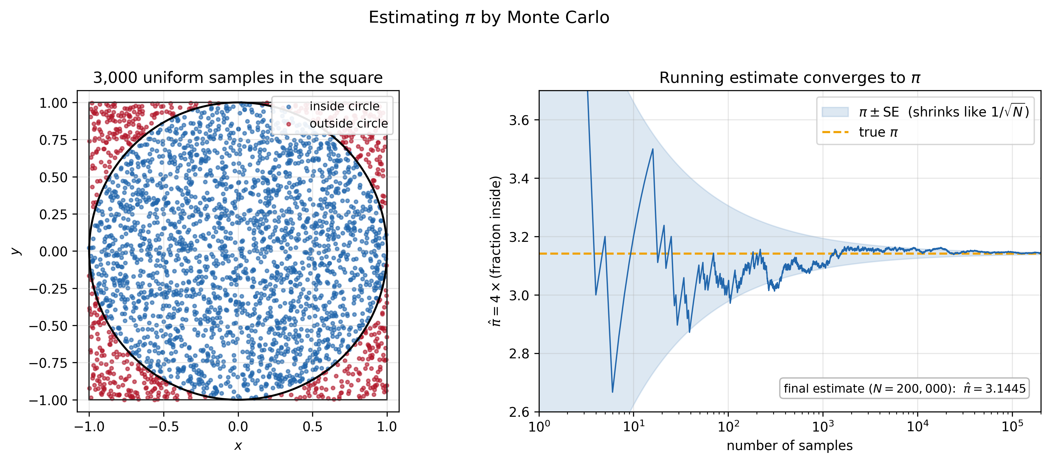
Consider the problem of estimating the area of the unit circle—which is just $\pi$. It’s given by the integral:

\[\int_{\text{circle}} 1 \, dx\, dy.\]

We can recast this as an expectation. Let $\mu$ be the uniform distribution on the $2\times 2$ square. Then:

\[\begin{align} \pi &= \int_{\text{circle}} 1 \, dx\, dy \\ &= 4\int \mathbf{1}_{x^2 + y^2 \le 1}\,\mu(dx,dy) \\ &= 4\,\mathbb{E}_{\mu}\!\left[\mathbf{1}_{x^2 + y^2 \le 1}\right]. \end{align}\]

The factor of $4$ is due to the area of the square. The expectation is just the probability that a uniform draw from the square lands inside the circle. Phrased this way, a recipe emerges: rather than computing the integral directly, we sample points from the square and count the fraction that land inside the circle. Multiply by four, and we have an estimate of $\pi$.

$Left: three thousand points sampled uniformly in the square, colored by whether they fall inside the inscribed circle. Right: the running estimate of pi---four times the fraction of points inside---converging to the true value as the sample count grows, inside a standard-error band that shrinks like one over the square root of N.$

In that problem we were sampling from the uniform distribution—which is easy. But what if we want to sample from some arbitrarily complicated distribution?

One of the simplest tools is Markov chain Monte Carlo (MCMC). The idea is to construct a Markov chain—a sequence of states in which the probability of the next state depends only on the current one, not on the entire past history—whose stationary distribution is the distribution we want to sample from.

You can think of Markov chain Monte Carlo as being inspired by the physical principle of ergodicity.

Ergodicity is the property that the time average along a single long trajectory equals the average over the whole ensemble. Equivalently: the fraction of time one realization spends in a region of state space equals the probability the ensemble assigns to that region. An example of an ergodic system is an ideal gas. At any given instant, the ensemble of gas molecules is uniformly distributed throughout the volume. But it’s also true that if you pick one molecule and follow it around for long enough, the trace of its trajectory will be uniformly distributed throughout the volume as well. That’s ergodicity.

This sounds almost trivial, but plenty of systems fail to be ergodic. If you wanted to estimate the distribution of adult heights, it would be no good to follow a single person around and record their height every morning—one trajectory never explores the ensemble. Ergodicity is exactly the condition that lets a single trajectory stand in for the whole population.

The Metropolis Algorithm

The Metropolis algorithm was the original physics-inspired sampling algorithm, invented by a team of physicists at Los Alamos in 1953 (Metropolis, Rosenbluth, Rosenbluth, Teller, and Teller). It relies on a Markov chain that we can follow—like a particle—in order to sample from a distribution. Assume that your distribution is of the form:

\[\pi(x) = \frac{e^{-V(x)}}{Z}\]

We will assume that we can query the potential $V(x)$ for any state.

The way the Metropolis algorithm works is that you have a proposal function $q(x,y)$. The proposal can be thought of as a conditional probability distribution: $q(x,y)$ gives, conditional on currently being at $x$, the probability of proposing a move to $y$. You want the proposal to be something simple that you can sample from—like a Gaussian.

\[q(x,y) = \frac{1}{\sqrt{2\pi}\,\sigma}\exp\!\left(-\frac{(y-x)^2}{2\sigma^2}\right)\]

Imagine you want to sample from the distribution depicted below and your sample from your proposal.

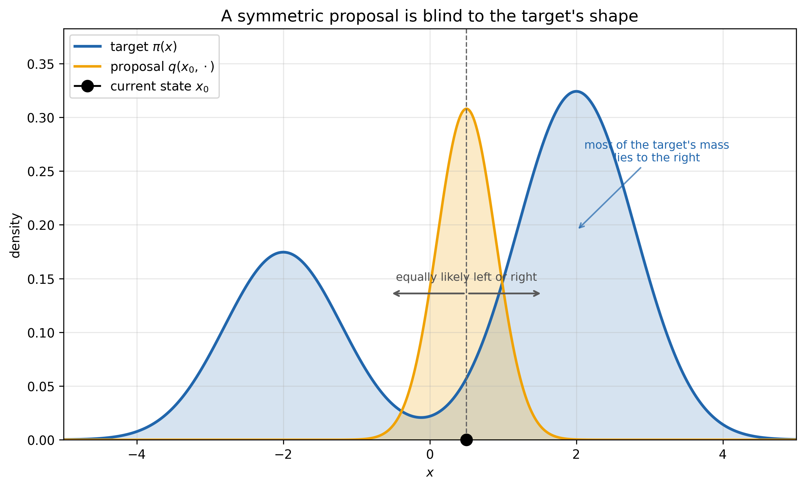
An asymmetric bimodal target density with the current state marked just right of center and a thin symmetric Gaussian proposal centered on it. The proposal is equally likely to step left or right, even though most of the target's probability mass lies to the right.

The problem is that the proposal is generic—it doesn’t adhere to the structure of the target. In the picture above, the proposal is symmetric about the current point, so we are equally likely to move left or right. But most of the target’s probability mass lies to the right, so a naive random walk that simply followed this proposal wouldn’t mix efficiently into the target’s steady-state distribution. We would ideally like to bias the proposal toward higher-probability regions—or at the very least, bias it locally in that direction.

The key to the Metropolis algorithm is that we don’t always accept the proposal. Given a proposal, if it would take you from a region of lower probability to one of higher probability (equivalently, from higher potential to lower potential), you always accept it. But if it would take you from higher probability to lower probability, you reject it with a probability that grows with the gap in energy between the two states: the more the proposal has you go “uphill”, the more likely you are to reject it.

The acceptance rule is chosen so that, in equilibrium, the flux of probability from $x$ to $y$ exactly balances the flux from $y$ to $x$.

\[\alpha(x,y) = \min\left\{\frac{\pi(y)\,q(x,y)}{\pi(x)\,q(y,x)},\; 1\right\}\]

where $\pi$ is the target distribution and $q$ is the proposal kernel. And notice: the acceptance ratio doesn’t require knowing the normalization constant $Z$. Since $\pi(x) = e^{-V(x)}/Z$, the two copies of $Z$ cancel:

\[\begin{align} \frac{\pi(y)\,q(x,y)}{\pi(x)\,q(y,x)} &= \frac{\big(e^{-V(y)}/Z\big)\,q(x,y)}{\big(e^{-V(x)}/Z\big)\,q(y,x)} \\ &= \frac{e^{-V(y)}\,q(x,y)}{e^{-V(x)}\,q(y,x)}. \end{align}\]

The acceptance rule above is actually the more general version. The original Metropolis algorithm (1953) required the proposal to be symmetric, $q(x,y) = q(y,x)$, so the proposal terms cancel and the acceptance ratio simplifies to $\min\{\pi(y)/\pi(x),\, 1\}$. The generalization to asymmetric proposals was made by Hastings in 1970, giving us what we now call the Metropolis-Hastings algorithm.

There are two main physical intuitions behind the Metropolis algorithm. The first is that probability distributions can be conceived as Boltzmann distributions—the distributions from physics that give the probability of a system occupying a given microstate at thermal equilibrium.

\[p(x) = \frac{e^{-E(x)/T}}{Z}\]

This distribution arises because a system in contact with a temperature bath minimizes its free energy, which trades off two competing objectives: lowering its energy and raising its entropy. The Boltzmann distribution is the compromise between them—lower-energy states are favored (which lowers the expected energy), but probability mass is still spread across many states (which raises the entropy).

The other physical intuition behind the Metropolis-Hastings algorithm is detailed balance. Detailed balance is the property that traversing a given sequence of microstates in reverse order is just as likely as visiting them in the forward order. In physics, this is sometimes called microscopic reversibility.

To understand detailed balance, consider two Markov chains on three states arranged in a triangle. In the first chain, at every step the system transitions to one of its two neighbors with equal probability $1/2$. If I hand you a sequence of states from this chain, you cannot tell a forward trajectory from a backward one—the transition probabilities are symmetric, so both directions are equally likely. This chain satisfies detailed balance.

Now consider a second chain where the system moves clockwise with probability $1/3$ and counterclockwise with probability $2/3$. Here, if I hand you a sequence of states, you can distinguish forward from backward—in the forward time direction, there is a clear counterclockwise drift. This chain violates detailed balance.

Two three-state Markov chains on a triangle with the same uniform stationary distribution. Left: each edge is traversed with probability one-half in both directions, satisfying detailed balance. Right: the chain drifts clockwise with probability two-thirds and counterclockwise with probability one-third, violating detailed balance.

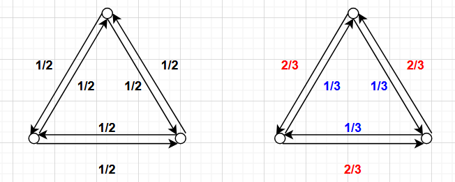
What’s interesting is that the long-run statistics of the two chains are identical: both spend equal time in each state (a uniform stationary distribution). The difference is that detailed balance gives us a much stronger guarantee about the dynamics.

For the Metropolis algorithm, what matters is not just that it converges to the right distribution, but that it does so in a time-reversible way. It’s this time-reversibility that makes it provably correct: if the transitions satisfy detailed balance with respect to the target distribution, then that distribution must be stationary under the dynamics.

Simulated Annealing

Recall that the Boltzmann distribution $p(x) \propto e^{-E(x)/T}$ depends on a temperature parameter $T$. At high temperatures, the distribution is nearly flat—every state has roughly the same probability. At low temperatures, the distribution concentrates sharply around the states of lowest energy.

Simulated annealing, proposed by Kirkpatrick, Gelatt, and Vecchi in 1983, exploits this observation. The idea is borrowed from metallurgy, where annealing refers to heating a metal to a high temperature and then slowly cooling it. At high temperature, the atoms are free to rearrange. As the temperature decreases, they settle into a low-energy crystalline structure. Cool too quickly and you get a disordered, high-energy amorphous solid. Cool slowly enough and the system finds its way to the global energy minimum.

The algorithm mirrors this physical process exactly. You start by running the Metropolis algorithm at a high temperature, where the chain moves freely and rarely gets stuck. Then you gradually decrease the temperature according to some cooling schedule. At each temperature, the chain samples from the corresponding Boltzmann distribution. As the temperature drops, the chain spends more and more of its time near the low-energy states, until eventually—if the cooling is slow enough—it concentrates on the global minimum.

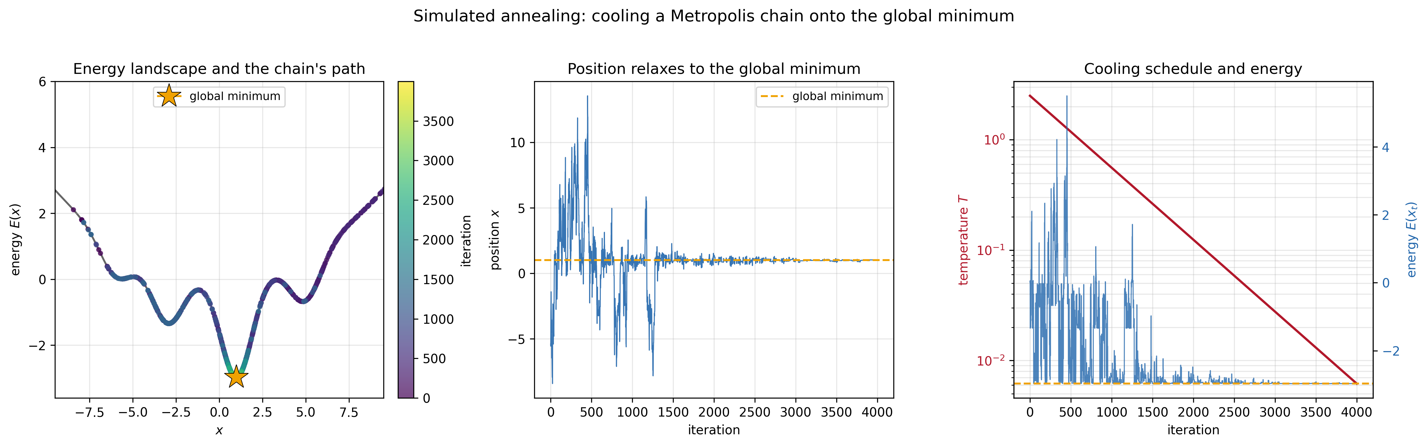
Left: a rugged one-dimensional energy landscape with several local wells and one deep global well, overlaid with the annealing chain's path colored by iteration. Middle: the chain's position over time, exploring widely at first and then relaxing onto the global minimum. Right: the geometric cooling schedule alongside the chain's energy settling to the global-minimum value.

What makes simulated annealing a powerful optimization technique is that it can escape local minima. At high temperatures, uphill moves are accepted with reasonable probability, letting the chain climb out of shallow energy wells. As the temperature decreases, escaping becomes harder, and the chain settles near what is hopefully the global minimum. This helps simulated annealing overcome a central weakness of greedy optimization methods (like gradient descent)—they can get trapped in the first local minimum they find.

Langevin Monte Carlo

In 1905, Albert Einstein had a pretty productive year.

He famously derived special relativity from just two axioms—that the speed of light is constant and that the laws of physics are the same in all inertial frames—and shortly thereafter used it to arrive at one of the most famous equations in science, $E=mc^2$. He also produced one of the earliest results in quantum mechanics, his explanation of the photoelectric effect (for which he would later receive the Nobel Prize).

Less well-known is that Einstein’s very first major contribution that year had nothing to do with relativity or quantum mechanics, but with statistical physics. If you look at a free-floating particle suspended in a liquid, it will jitter, moving in a herky-jerky fashion. This was explained by Einstein in 1905 as Brownian motion.

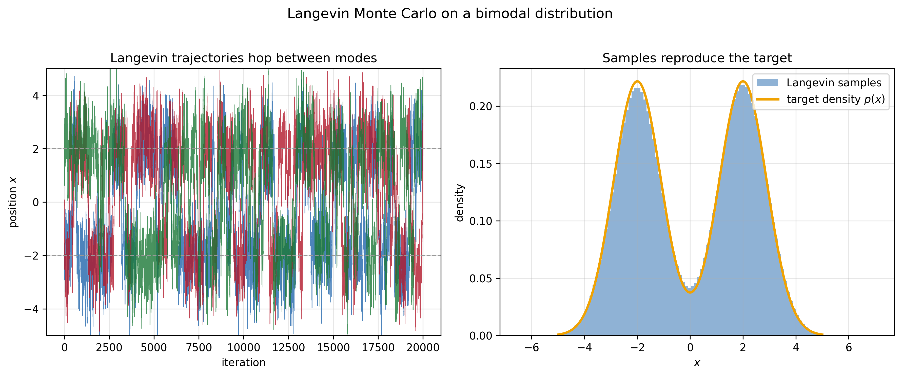
This was then made mathematically precise by Paul Langevin in 1908. Decades later, that same equation was repurposed as a sampler. The recipe, now called Langevin Monte Carlo, turns the physics of a particle diffusing in a potential into a way of drawing samples: given a distribution $p(x) \propto e^{-V(x)}$, the SDE

\[dX_t = -\nabla V(x) \,dt + \sqrt{2}\,dW_t\]

has $p$ as its stationary distribution.

The intuition behind Langevin Monte Carlo is very similar to the one behind the Metropolis-Hastings algorithm: the drift term biases the dynamics toward higher-probability regions, while the Brownian noise supplies enough randomness for the system to keep exploring the state space.

Left: three Langevin trajectories sampling a bimodal target, jittering within each mode and occasionally hopping across the barrier between the two modes at plus and minus two. Right: a histogram of the Langevin samples overlaid on the true bimodal density, which it reproduces closely.

Langevin Monte Carlo feels physics-inspired in two ways. First, it has deep ties to a piece of statistical-mechanics history (the Langevin equation). And second, it feels embodied. You can imagine carrying out this sampling algorithm in the real world—you set up a particle in a potential trap, let it jitter for a little while, and then record its location.

Hamiltonian Monte Carlo

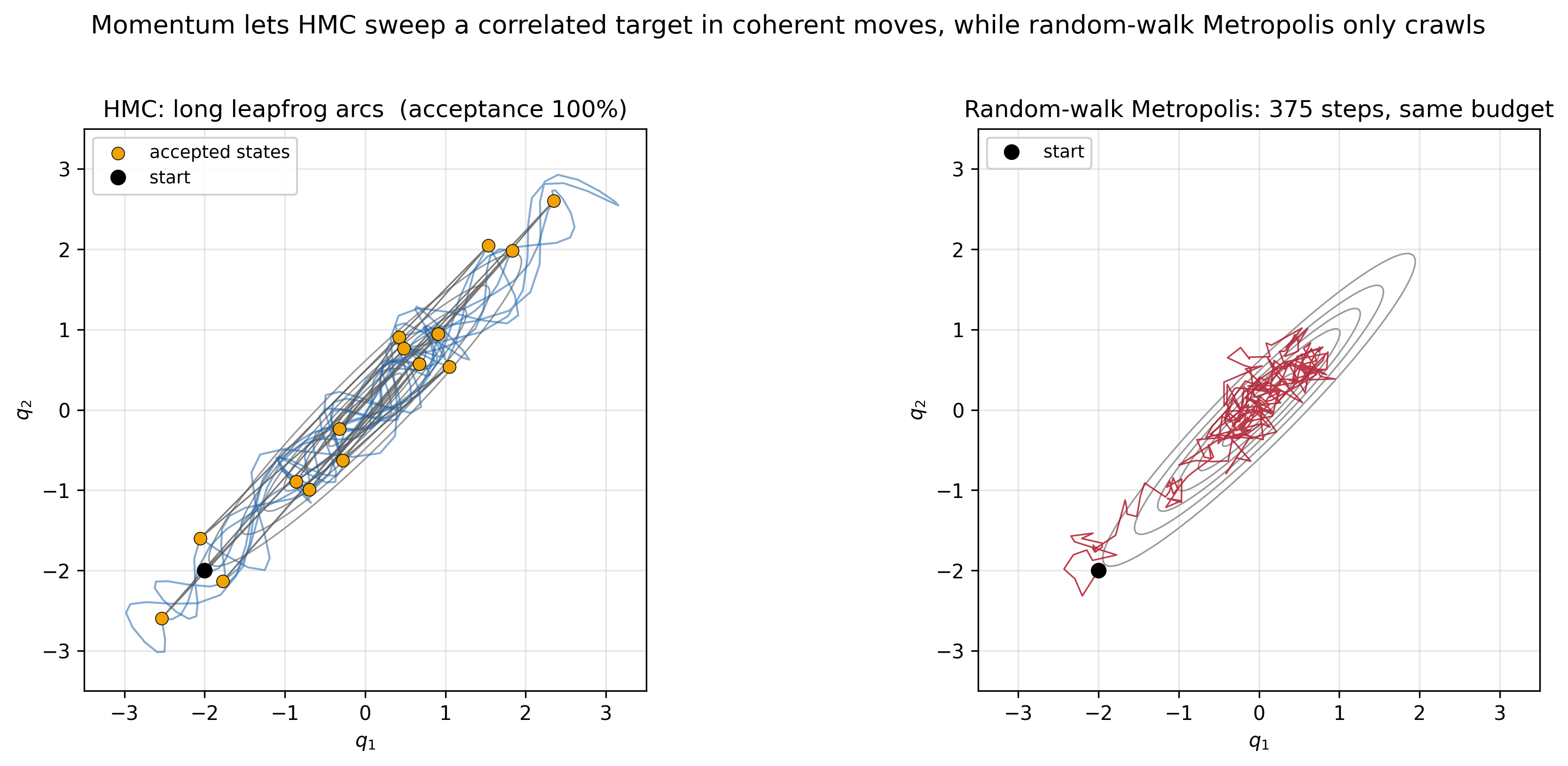
Langevin dynamics gives us a way to use gradient information to sample, but it has a limitation: because it is a first-order method (no momentum), it explores the state space via a biased random walk—which can be slow.

Hamiltonian Monte Carlo (HMC), introduced by Duane, Kennedy, Pendleton, and Roweth in 1987, solves this problem by borrowing a deeper piece of physics: Hamiltonian mechanics. It was originally invented for lattice quantum chromodynamics calculations and was later popularized in statistics by Radford Neal. Today it is the workhorse behind probabilistic programming languages like Stan. With HMC, we augment the position state space with auxiliary momentum variables. Then we take advantage of the energy-conserving properties of Hamiltonian dynamics in order to efficiently explore the state space.

Recall from classical mechanics that a Hamiltonian system is described by a pair of variables: a position $q$ and a momentum $p$. The total energy (the Hamiltonian) is the sum of the kinetic and the potential energy:

\[H(q, p) = V(q) + \frac{1}{2}p^T M^{-1} p,\]

where $M$ is a mass matrix and $V(q)$ is the potential energy (which will correspond to the negative log probability density of our target distribution). Hamilton’s equations of motion tell us how the system evolves:

\[\frac{dq}{dt} = M^{-1} p, \qquad \frac{dp}{dt} = -\nabla V(q).\]

The key physical insight is that Hamiltonian dynamics are energy-preserving and volume-preserving in phase space (Liouville’s theorem). This means that if we simulate these dynamics exactly, we can propose large moves in the state space that are accepted with probability one—because the total energy, and hence the target density in the augmented space, is unchanged. (In practice the integrator is only approximate, so a small correction is needed.) Rather than taking small, diffusive steps like a random walk, the momentum carries the state along level sets of the Hamiltonian, sweeping through the target distribution in long, coherent arcs.

In practice we can’t simulate continuous Hamiltonian dynamics exactly, so we use a numerical integrator. The standard choice is the leapfrog integrator, which alternates half-steps in momentum with full steps in position:

\[p_n\!\left(t + \tfrac{\Delta t}{2}\right) = p_n(t) - \tfrac{\Delta t}{2}\,\nabla V(x)\big|_{x = x_n(t)}\] \[x_n(t + \Delta t) = x_n(t) + \Delta t\, M^{-1}\, p_n\!\left(t + \tfrac{\Delta t}{2}\right)\] \[p_n(t + \Delta t) = p_n\!\left(t + \tfrac{\Delta t}{2}\right) - \tfrac{\Delta t}{2}\,\nabla V(x)\big|_{x = x_n(t + \Delta t)}\]

The leapfrog integrator is symplectic: it preserves the geometric structure of Hamiltonian dynamics even though it introduces small energy errors. Those errors are corrected by a Metropolis acceptance step at the end.

The full HMC algorithm is:

Resample momentum: draw a fresh momentum $p \sim \mathcal{N}(0, M)$.
Simulate dynamics: run $L$ steps of leapfrog integration to get a proposed state $(q’, p’)$.
Accept or reject: accept the proposal with probability $\min\{1,\, e^{-[H(q’, p’) - H(q, p)]}\}$.
Repeat from step 1.

Left: Hamiltonian Monte Carlo on a strongly correlated two-dimensional Gaussian; leapfrog trajectories sweep in long coherent arcs along the correlation ridge, with accepted states marked. Right: random-walk Metropolis given the same computational budget, crawling slowly near its starting point and barely exploring the target.

The physical picture is vivid: imagine placing a ball on a hilly landscape and giving it a random kick. The ball rolls along the landscape, trading kinetic energy for potential energy and back again, exploring the probability distribution by moving along level sets of the Hamiltonian. After some time, we stop the simulation, record the position, and repeat.

Diffusion Models

The most recent example I want to cover is diffusion models, introduced by Sohl-Dickstein, Weiss, Maheswaranathan, and Ganguli in 2015, drawing on principles from non-equilibrium statistical mechanics. The approach was later refined into the practical “Denoising Diffusion Probabilistic Models” (DDPM) by Ho, Jain, and Abbeel in 2020, which sparked the current ubiquity of diffusion models.

The way a diffusion model works is that, during training, you hand it an image and gradually add noise until the image is completely degraded—random white pixel noise. It is then the network’s job to predict what the noise was at the previous time step, given the current corrupted image.

A possible reason why diffusion models work so well is that they let different parts of the denoising process learn different levels of the image. The earliest denoising steps turn the random field into high-level features—rough shapes, composition, color palettes. Each subsequent step then adds finer and finer detail, until finally you have an image that should be a sample from the same distribution as natural images.

From a more formal perspective, diffusion models are an example of a score-based generative model: a generative model that aims to learn the score function, the gradient of the log probability density.

\[\text{score} = \nabla \log p(x)\]

For diffusion models specifically, the neural network learns the score functions of the intermediate distributions—the increasingly blurred versions of the data. Once you have the score at each noise level, you can reverse the diffusion process by running a time-reversed stochastic differential equation. This connection is what makes diffusion models a natural descendant of Langevin Monte Carlo.

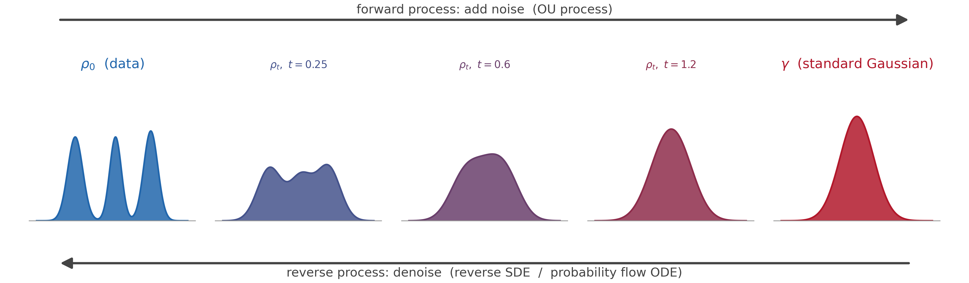
A trimodal data distribution morphing into a standard Gaussian under the forward noising process, with arrows marking the forward (noising) and reverse (denoising) directions.

The original 2015 paper frames the forward noising process as a non-equilibrium thermodynamic trajectory—a system driven away from equilibrium by the gradual addition of noise. The reverse process is then a way of learning the “thermodynamic” path back to the data distribution. While equilibrium statistical mechanics reasons about steady-state distributions, non-equilibrium statistical mechanics gives us tools to reason about the path between distributions—which is exactly what diffusion models exploit.