Probability Flow ODE Explained
Diffusion models are a type of generative model: machine learning models whose task is to generate a sample from a target distribution.
Imagine you would like a diffusion model that can generate images from the distribution of natural images. To train a diffusion model, you take real images and add noise to them. The model then has to try to denoise the corrupted image. Once the model is trained, you can hand it pure pixel noise—one that was never produced by corrupting any real image—and the model will attempt to “denoise” it, generating a fresh sample from the distribution it was trained on.
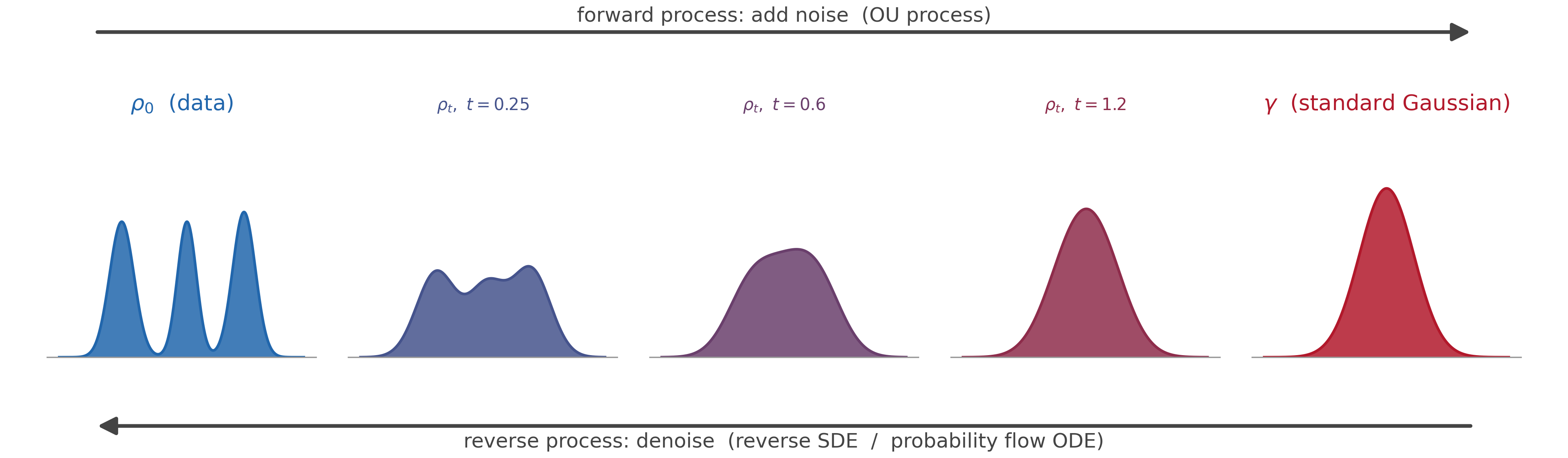
Mathematically, this is all most naturally described in the language of stochastic differential equations. A common choice for the noising process is the Ornstein-Uhlenbeck process (OU process). The OU process combines a linear restoring force—mathematically identical to the force exerted by an ideal spring—with Brownian noise. Its stationary distribution is the standard Gaussian.
\[dX_t = -X_t\, dt + \sqrt{2}\, dW_t\]The most natural way to think about the sampling process is to define the corresponding reverse SDE: a stochastic differential equation whose process $X_t^{\leftarrow}$ runs from the standard Gaussian back to the data distribution. The reverse SDE looks a lot like the forward one—with two major differences. First, the restoring force flips sign—instead of pulling inward toward the origin, it now pushes outward. Second, we pick up an additional “entropic force” proportional to the score function—the gradient of the log probability density—of the marginal distributions of the forward process. This is why diffusion models fall under the umbrella of score-based generative models.
\[dX_t^{\leftarrow} = \big(X_t^{\leftarrow} + 2\, \nabla \log \rho_{T-t}(X_t^{\leftarrow})\big)\, dt + \sqrt{2}\, dW_t\]Here $\rho_t$ is the marginal density of the forward process at time $t$. The reverse process runs over $t \in [0, T]$, starting from (approximately) the standard Gaussian and ending at the data distribution $\rho_0$. You can integrate it to sample from the target distribution.
But the reverse SDE is not perfect. Simulating an SDE is computationally expensive, since the noise forces you to discretize finely in time. Thankfully, there is an alternative. Rather than the reverse SDE, you can use an ordinary differential equation that has the same marginals—the same distribution at every time—even though its trajectories are deterministic. This is called the probability flow ODE.
Deriving the Reverse SDE
Let’s set up some notation. The forward process $X_t$ has marginal density $\rho_t$, with $\rho_0$ denoting the data distribution. Running the OU process noises the data over time until, in the limit of infinite time, $\rho_t \to \gamma$, the standard Gaussian.
We denote the reverse process by $X_t^{\leftarrow}$ and run it forward over $t \in [0, T]$ for a large final time $T$ (at which $\rho_T \approx \gamma$). The reverse process at its time $t$ visits the forward marginal $\rho_{T-t}$: it starts at $\rho_T \approx \gamma$ and ends at $\rho_0$.
We would like to derive the reverse SDE—the dynamics that carry $\gamma$ back to $\rho_0$. But how do we do that?
The trick is to pass through the Fokker-Planck equation. It’s worth noting that this reverses the usual workflow: ordinarily we start with a Fokker-Planck equation describing how a density ought to evolve and then derive an SDE we can simulate from. Here we go the other way. We start with the SDE, derive its corresponding Fokker-Planck equation, reverse time at the level of the density, and only then turn the result back into an SDE.
In general, every SDE has a corresponding Fokker-Planck equation governing the evolution of its density, and vice versa:
\[dX_t = b(X_t)\, dt + \sqrt{2D}\, dW_t \qquad \Longleftrightarrow \qquad \partial_t \rho_t = -\nabla \cdot (b\, \rho_t) + D\, \Delta \rho_t\]For the OU process we have $b(x) = -x$ and $D = 1$. Equivalently, $b = -\nabla V$ with $V(x) = \tfrac{1}{2}\lVert x \rVert^2$: the OU process is just Langevin dynamics in a quadratic “spring” potential. Its Fokker-Planck equation is therefore:
\[\partial_t \rho_t = \nabla \cdot (x\, \rho_t) + \Delta \rho_t\]The drift term $\nabla \cdot (x\, \rho_t)$ pulls probability mass inward toward the origin, while the diffusion term $\Delta \rho_t$ spreads it out. The standard Gaussian is the steady state at which the two balance.
Now we will reverse time. Recall that the reverse process visits the forward marginals in reverse order: $\rho_{T-t}$. By the chain rule, reversing time flips the sign of the time derivative, so the reverse-time density evolves by negating the right-hand side of the forward equation:
\[\partial_t \rho_{T-t} = -\nabla \cdot (x\, \rho_{T-t}) - \Delta \rho_{T-t}\]Notice the sign of the diffusion term: it is now negative. This is the backward heat equation, and it is famously ill-posed—you cannot simply run diffusion in reverse. So while this equation is correct, it is not yet something we can simulate. We need to massage it back into the form of a genuine Fokker-Planck equation, with a positive diffusion term.
The key is an identity that converts the Laplacian into a divergence using the score. Since $\nabla \log \rho = \nabla \rho / \rho$, we have $\rho\, \nabla \log \rho = \nabla \rho$, and therefore:
\[\begin{align} \Delta \rho_{T-t} &= \nabla \cdot (\nabla \rho_{T-t}) \\ &= \nabla \cdot (\rho_{T-t}\, \nabla \log \rho_{T-t}) \end{align}\]We can then split the negative diffusion term into two parts:
\[-\Delta \rho_{T-t} = -2 \Delta \rho_{T-t} + \Delta \rho_{T-t}\]Then we use the identity above to rewrite the first piece as a drift and keep the second as a positive diffusion term:
\[\partial_t \rho_{T-t} = -\nabla \cdot \big[(x + 2\, \nabla \log \rho_{T-t})\, \rho_{T-t}\big] + \Delta \rho_{T-t}\]This is now a bona fide Fokker-Planck equation, with drift $x + 2 \nabla \log \rho_{T-t}$ and $D = 1$. Reading off the corresponding SDE via the correspondence above gives the reverse SDE:
\[dX_t^{\leftarrow} = \big(X_t^{\leftarrow} + 2\, \nabla \log \rho_{T-t}(X_t^{\leftarrow})\big)\, dt + \sqrt{2}\, dW_t\]The Probability Flow ODE
But let’s back up to the reverse-time Fokker-Planck equation and make a different choice. Instead of keeping a leftover diffusion term, we can absorb all of it into the drift. Applying the same identity $\Delta \rho_{T-t} = \nabla \cdot (\rho_{T-t}\, \nabla \log \rho_{T-t})$ to the lone diffusion term, we get:
\[\partial_t \rho_{T-t} = -\nabla \cdot \big[(x + \nabla \log \rho_{T-t})\, \rho_{T-t}\big]\]There is no diffusion term left. This is a pure continuity equation.
\[\partial_t \rho_{T-t} = -\nabla \cdot (\rho_{T-t}\, v_t)\]where the velocity field is given by:
\[v_t(x) = x + \nabla \log \rho_{T-t}(x)\]A continuity equation describes a density carried along by a deterministic velocity field—probability mass simply flows. So we can read off an ODE for the trajectory of each particle:
\[\frac{dX_t^{\leftarrow}}{dt} = X_t^{\leftarrow} + \nabla \log \rho_{T-t}(X_t^{\leftarrow})\]This is the probability flow ODE. Compare it with the reverse SDE: the drift is identical except that the score now enters with coefficient $1$ instead of $2$—exactly half. Therefore, if you learn the score function, then you can simulate both the reverse SDE and the probability flow ODE.
There is a clean way to read the velocity field. Because $\gamma$ is the standard Gaussian, $\nabla \log \gamma(x) = -x$, so the restoring term $x$ is just $-\nabla \log \gamma$. The two pieces of the velocity then collapse into a single gradient:
\[\begin{align} v_t(x) = \nabla \log \rho_{T-t}(x) - \nabla \log \gamma(x) = \nabla \log \frac{\rho_{T-t}}{\gamma}(x) \end{align}\]The flow is driven by the gradient of the log-density-ratio between the current marginal and the standard Gaussian.
Conceptually, the Fokker-Planck equation only constrains the evolution of the density. It is agnostic about whether that density is realized by stochastic SDE dynamics or by deterministic ODE pushforward. This is why the probability flow ODE has the same marginals as the reverse SDE—and therefore the same marginals as the forward noising process. However, the two differ at the level of trajectories: the reverse SDE matches the forward process as a path measure, reproducing its full joint statistics across time, whereas the probability flow ODE matches only the marginals, while following its own smooth deterministic paths.
This also reveals that there were never just two choices. How much of the score to keep as drift versus diffusion was arbitrary. Reintroducing diffusion of strength $\sqrt{2\lambda}$, compensated by an extra $\lambda\, \nabla \log \rho_{T-t}$ in the drift, gives a one-parameter family of dynamics, all sharing the same marginals:
\[dX_t^{\leftarrow} = \big(X_t^{\leftarrow} + (1 + \lambda)\, \nabla \log \rho_{T-t}\big)\, dt + \sqrt{2\lambda}\, dW_t, \qquad \lambda \in [0, 1]\]At $\lambda = 1$ we recover the reverse SDE. At $\lambda = 0$, the diffusion vanishes and we are left with the probability flow ODE. In the diffusion-model literature, this is the family interpolating between stochastic, DDPM-style ancestral sampling and the deterministic DDIM sampler.
The probability flow ODE does more than generate samples—it defines a map. Each starting point is deterministically transported along the flow, so integrating from $\gamma$ all the way to $\rho_0$ (in the idealized $T \to \infty$ limit, where the forward process fully relaxes to the Gaussian) gives a single deterministic map that pushforwards the standard Gaussian onto the data distribution.
This map is known as the Kim-Milman map, or the reverse heat flow map.
(A brief note on jargon: “probability flow ODE” is the term of choice in the machine learning community, whereas in the more math-heavy, optimal-transport-adjacent communities the same object is usually called the Kim-Milman or reverse heat flow map.)
The map is special on two counts. Practically, the probability flow ODE is far nicer to work with than the reverse SDE: it is deterministic, and you can integrate it with off-the-shelf, large-step ODE solvers rather than finely discretized stochastic steps. Theoretically, the Kim-Milman map is one of the very few maps between distributions—the optimal transport map being the other—whose properties we understand well enough to prove substantial results about.