The Score Is Just The Force
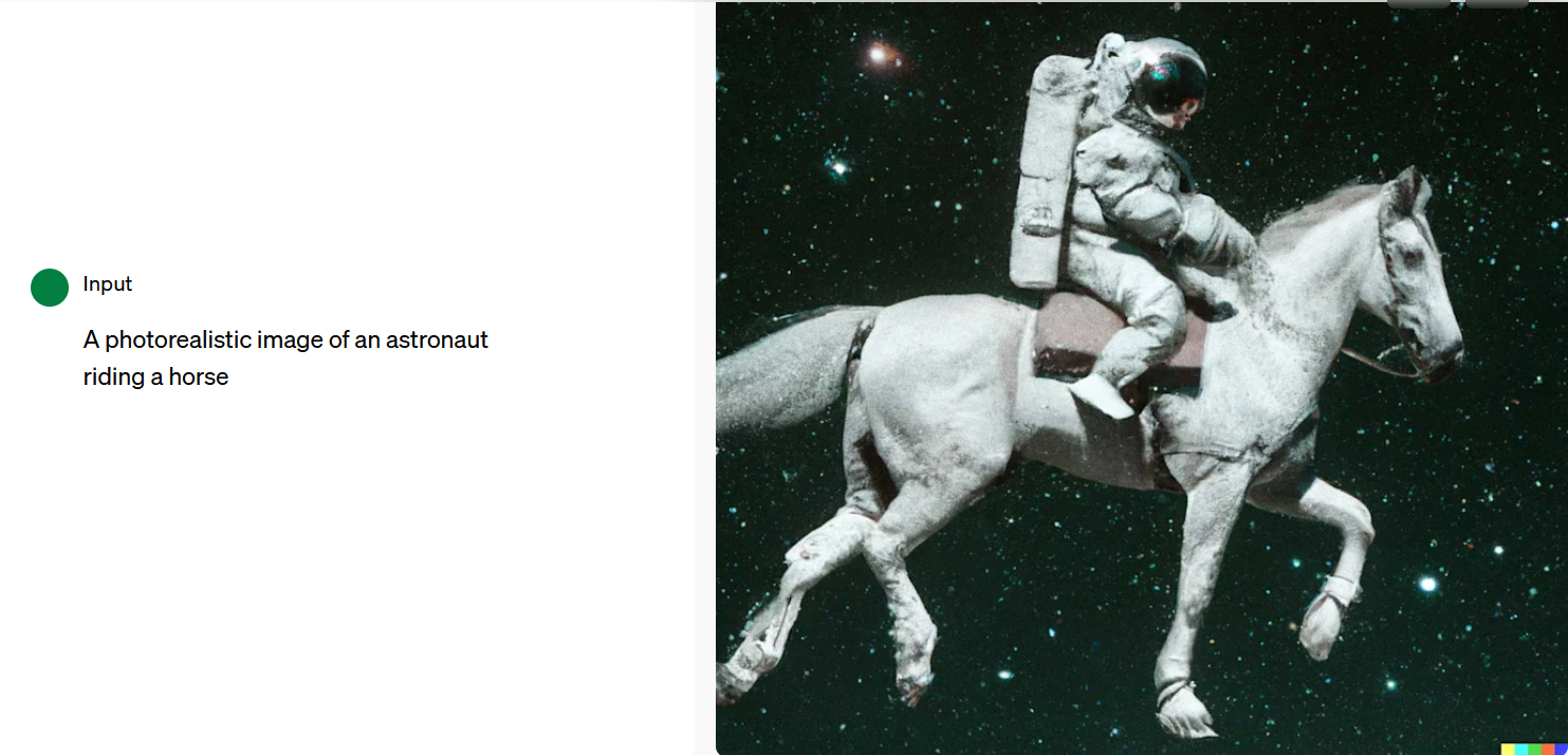
In machine learning, a generative model aims to learn the underlying distribution $p(x)$ of the data. This contrasts with supervised learning models (also called discriminative models) that map inputs to specific outputs. For example, DALLE-2 is a generative model that creates new images, while Inception v4 is a discriminative model that classifies images into predefined categories.

Among the many flavors of generative models, score-based generative models have recently gained in popularity. These models learn something called the score function—the gradient of the log probability density:
\[s = \nabla \log p(x)\]The name “score” is rather obscure and doesn’t help build intuition. It also doesn’t help that the definition of the score as used by the machine learning community is slightly different than the original definition from statistics. In statistics, the score is the gradient of the log probability density with respect to the parameters, not the underlying space.
But the score has a straightforward physical interpretation: the score is just the force.
Assume we have a probability distribution that can be represented as a Gibbs measure: $p(x) = \frac{e^{-V}}{Z}$, where $V$ is the potential and $Z$ is the partition function. Taking the log of the probability gives us (up to a constant) the negative potential: \(\log p(x) = -V(x) - \log Z\)
This connection to physics isn’t just mathematical coincidence—it’s fundamentally useful. Energy-based models exploit this relationship by directly parametrizing an energy function $E(x)$ that plays the role of the potential $V(x)$. Extending the analogy, since $\nabla \log p(x) = -\nabla V(x)$, the score is exactly the force! Perhaps we should call these “force-based generative models” instead.

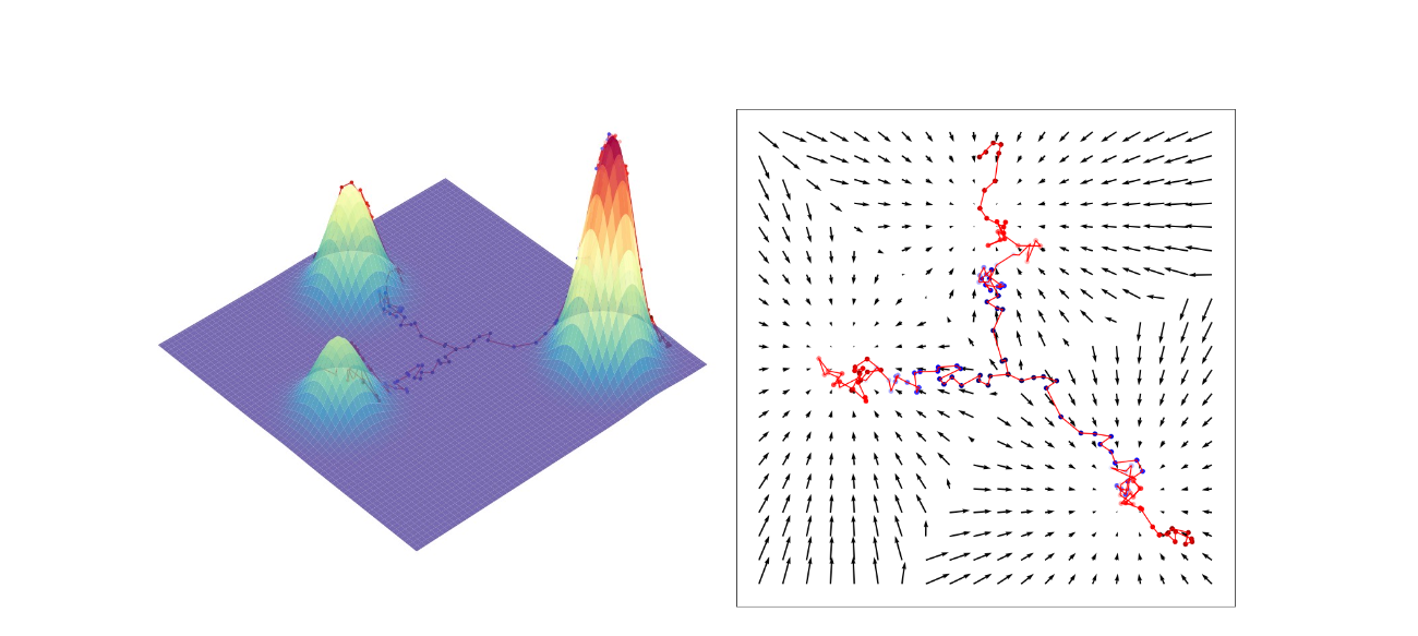
In the physical world, particles tend to gather in regions of lower potential energy because forces push them towards local minima, fighting against random thermal fluctuations. Our generative models are doing exactly the same thing—using the learned force field to push samples towards regions of high probability. This physical interpretation helps explain the strengths and weakness of the score functions: forces capture local information about the probability landscape.
There’s an elegant connection to Langevin dynamics. One can ask: once you’ve learned the score function, how do you actually use it to sample from your distribution? Consider the stochastic differential equation:
\[dX_t = -\nabla V dt + \sqrt{2} \ dW_t\]This equation describes a particle moving under two influences: a force term ($-\nabla V$) and random noise ($dW_t$). The steady-state distribution of this process is exactly the Gibbs measure $e^{-V}$.
Traditional Langevin sampling assumes we already know the potential gradients, focusing instead on questions like convergence speed to steady state. The key insight of score-based generative modeling is that for an unknown distribution, we can use a neural network to learn these potential gradients.
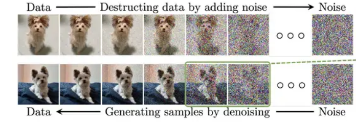
The force analogy, while becoming more subtle, remains useful when considering diffusion models. In these models, we begin with an image and gradually add noise until it becomes pure random static. We then train a neural network to reverse this process and recover the original image. The key difference is that instead of working with a single static probability distribution, we work with a series of distributions indexed by the time step of the diffusion process. The initial distribution represents natural images, while the final distribution is a standard Gaussian distribution in pixel space.

How does the neural network learn to deblur the image? And how does this connect to the score function? The intuition is that given your current position in pixel space, the previous point in pixel space was likely to be: (1) nearby and (2) high in probability. Therefore, when reversing the noise process, the neural network must learn to push samples towards local probability maxima for the previous distribution. This is given precisely by the score function of the distribution at the previous time step.