Towards a Classical Mechanics of Machine Learning
The connection between statistical physics and machine learning is well-established by now—so much so that the 2024 Nobel Prize in Physics went to John Hopfield and Geoffrey Hinton for foundational, statistical-physics-inspired contributions to the field.
And it doesn’t stop there. Statistical physics has seeded an enormous amount of modern machine learning:
- The partition function. Generative models are plagued by the intractability of the normalization constant—the very same object as the partition function $Z$ in statistical physics.
- Langevin dynamics. Optimization and sampling are routinely cast as noisy gradient flow—a particle diffusing in a potential.
- Diffusion models. The denoising-diffusion framework was inspired by non-equilibrium thermodynamics, drawing on ideas like Jarzynski’s equality.
- Dynamical mean-field theory. Borrowed from the study of disordered systems, it is now used to track the high-dimensional dynamics of learning.
But what I find striking is that the ideas of classical mechanics have not had the same penetrance as those of statistical mechanics.
That’s not to say they’re absent. When we train a neural network, we write down a loss function and then let the parameters evolve in order to minimize it. At its core, optimization is a generalization of the oldest intuition in mechanics—that a ball released on a hillside rolls down the slope and comes to rest at the bottom. And since classical mechanics is the physics of how systems move and evolve in time, you might expect it to have a great deal to say about the dynamics of learning.
Here’s an example. The most common improvement on vanilla gradient descent is momentum. Gradient descent updates the parameters using only the gradient at the current point. A momentum method instead maintains a velocity that accumulates past gradients and steps along that. For heavy-ball momentum, the updates read:
\[\begin{align} v_{t+1} &= \beta v_t - \eta\, \nabla L(x_t) \\ x_{t+1} &= x_t + v_{t+1} \end{align}\]Just as a rolling ball builds up speed, the parameters now carry inertia.
But there are deeper ideas in classical mechanics. At the undergraduate level, classical mechanics is the study of forces and the differential equations they produce. In its more advanced form, the whole subject is reorganized around Lagrangians and Hamiltonians, conserved quantities, symmetries, and the geometry of phase space. It is this second, more abstract layer that has found little purchase in machine learning. To be fair, there are scattered works in this vein—for instance, this elegant paper on a variational perspective on acceleration—but nothing on the scale of the statistical-physics borrowings.
So if optimization is a kind of mechanics, why have Lagrangians, Hamiltonians, and conserved quantities not become standard tools the way partition functions and Langevin dynamics have? My sense is that the machinery of classical mechanics was built for the physics of the real world, and the physics of machine learning differs from it in three important ways—each of which violates an assumption the classical toolkit leans on. In machine learning:
-
The dynamics are dissipative rather than conservative.
-
The landscape is badly non-convex, because the interactions are unknown rather than fixed by a few known laws.
-
The dynamics operate in discrete rather than continuous time.
The first difference is that real-world dynamics conserve energy, whereas optimization is about minimizing it. Many of the most powerful results in classical mechanics rest on conserved quantities—above all conservation of energy, the shadow of time-translation symmetry. Other symmetries buy other conserved quantities: momentum from spatial translation symmetry, angular momentum from rotational symmetry. These are what make hard problems tractable, pinning a trajectory to a lower-dimensional surface in phase space and letting you integrate the motion. Optimization has nothing of the kind. The loss is engineered to decrease—that is the whole point—so the dynamics are dissipative: energy bleeds out of the system on its way to a minimum. There is no conserved quantity to lean on.
The second difference is subtler: in physics we know the interactions, and in machine learning we don’t. In the real world there are a handful of fundamental interactions—gravity, electromagnetism, etc.—each with a known functional form. Solving a particular problem is then mostly a matter of specifying the initial distribution of mass and charge. Crucially, the potential decomposes into physically meaningful pieces:
\[V(x) = V_{\text{gravity}} + V_{\text{electromagnetism}} + \cdots,\]and each piece carries its own structure that we know how to exploit. The loss function of a machine-learning model plays the role of the potential, but its shape is dictated entirely by the data distribution. Consider the MSE loss:
\[L(w) = \frac{1}{n} \sum_{i=1}^n \big(f(x_i; w) - y_i\big)^2 = \frac{1}{n}\sum_{i=1}^n \ell_i(x_i, y_i, w).\]We could decompose the loss into one interaction term $\ell_i$ per data point, so that each example exerts its own pull on the parameters and the total loss is the average of those pulls. But that is a decomposition by data point, not by physics. We have no principled way to break the loss into a few interpretable terms with known structure, the way physics splits a potential into gravity plus electromagnetism. Doing so would require knowing in advance which structures in the data actually matter. And it is precisely this absence of known structure that leaves the loss landscape so badly non-convex: with no symmetries to organize it and no clean separation into simple parts, what we are left with is a high-dimensional surface full of valleys, ridges, and saddles that we must navigate essentially blind.
The third difference is that the physical world runs in continuous time, while optimization proceeds in discrete steps of some finite step size. Continuous time is where our cleanest theoretical tools live. There, gradient descent becomes the gradient flow, and the loss is a Lyapunov function for it—a quantity guaranteed to decrease monotonically along every trajectory. In discrete time, we lose that guarantee unless the step size is sufficiently small—much smaller than the step sizes actually used in practice. At any finite step size, the discretization and the local curvature of the loss interact in complicated ways: step too large relative to the curvature, and the loss can increase. The story is similar for conservative systems: a careless discretization will no longer conserve energy. Discrete time frequently invalidates the assumptions underlying both the dissipative and the conservative pictures.
None of these three difficulties is fatal on its own. In fact, relax any one of the three and a mature body of theory is waiting.
Relax the discreteness—work in continuous time—and you are back in the world of gradient flow, where the loss is a Lyapunov function and dissipative dynamics on even a non-convex landscape are well understood.
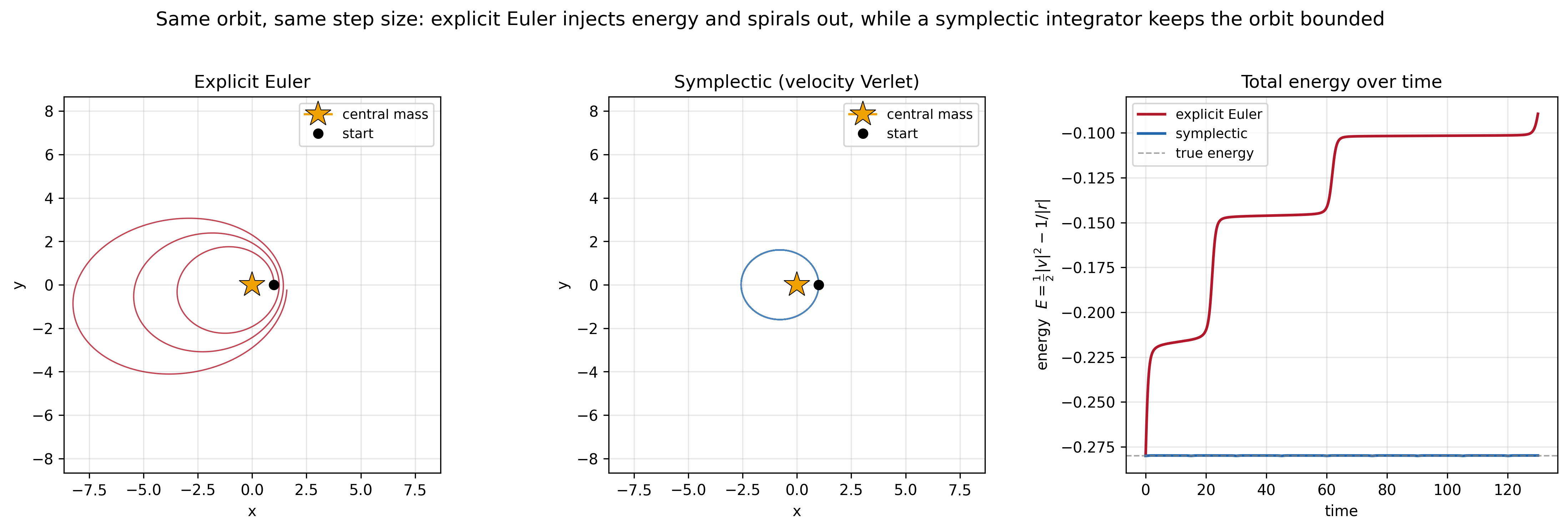
Relax the dissipation—conservative dynamics in discrete time—and you enter the realm of geometric integration. Here the goal is to design clever discretizations—symplectic integrators—that nearly conserve energy over astronomically long horizons, even though no finite-step scheme conserves it exactly. A naive Euler discretization of a planetary orbit slowly spirals in or out as energy drifts. A symplectic integrator keeps the orbit stable essentially forever, by respecting the geometric structure of phase space that the naive discretization ignores.
Relax the non-convexity—assume the landscape is convex—and you have convex optimization. It tells you how small a step you must take to be sure the loss goes down each iteration: roughly, the step size has to be inversely proportional to the curvature.
A genuine classical mechanics of machine learning would have to operate in the regime no existing theory fully covers: dissipative, discrete-time, and non-convex—all at the same time.