Phase Transitions As Fixed Points
Last year, I wrote about how phase transitions can be understood through the lens of global optimization. The thesis of the post was that phase transitions are the result of thermodynamic systems acting as solvers of global optimization problems: small changes in external conditions (which can be viewed as small perturbations of the free energy landscape) can result in large changes in the location of the argmin.
While I still think that framework is useful, I’ve been somewhat dissatisfied with it ever since. To apply it in other contexts, you have to assume that the system in question is capable of finding the global minimum of the objective—an assumption which is not always realized, even in some idealized sense, in many systems we colloquially describe as exhibiting phase transitions. In particular, I’ve had trouble fitting the phase transitions that have been empirically observed in machine learning into the global optimization framework, despite the fact that one of the defining features of machine learning is that the training objectives are highly non-convex.
This has led me to an alternative perspective: phase transitions as fixed points. Given a dynamical system, the phases of the system can be identified with the fixed points of the dynamics. The phase of a point is the fixed point that it gets mapped to in the limit of infinite time. A phase transition corresponds to either a small perturbation in the initial conditions or a small perturbation in the dynamics themselves that causes the system to end up at a different fixed point.
The main difference between the two frameworks is that global optimization is a static picture: we assume that the system will find itself in the global minimum, but there is no attempt to explain why or how that happens. The fixed point perspective is a dynamical picture: we have a specific process that governs the system’s time evolution, and we ask where that process takes us. In thermodynamic systems, the static picture seems reasonable because the size of the system means that the effective timescale to reach equilibrium is extremely fast relative to the timescale of our observation (though there are notable exceptions, such as spin glasses). But in many other contexts, it becomes important that we analyze the process of minimizing the objective, explicitly.
The “Phase Transitions As Fixed Points” perspective is not at all new. In his famous paper where he introduced the renormalization group, Ken Wilson includes a diagram of a non-convex landscape. He makes the point that, given two stable fixed points, there is a phase transition when your initial condition crosses from one basin of attraction to another. If you start on the left, you will eventually settle down at $x_A$. If you start on the right, you will eventually settle down at $x_B$.
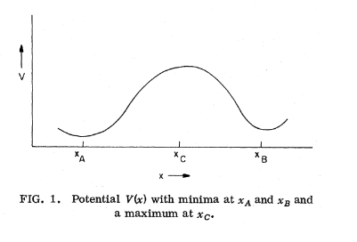
As Wilson succinctly put it himself: “The basic proposal of this paper is that the singularities at the critical point of a ferromagnet can be understood as arising from the $t=\infty$ limit of the solution of a differential equation.”
Let’s try to make this a bit more precise. Given an ODE, we can define the flow map $\phi_t(x)$. The flow map is a function that takes an initial condition $x$ as input and returns the location that the point will end up at after time $t$ following the dynamics of the ODE. The eventual fixed point that a point ends up at we can define as $\phi_\infty(x)$—this function maps every point in space to its eventual resting place.
It’s also helpful to consider not just one ODE, but a parametric family of ODEs. Each member of the family has an associated flow map. We can then think of the eventual fixed point as a function of both the starting point and the parameters:
\[\phi_\infty: D \times \Theta \rightarrow D\]where $D$ is the domain of the ODE and $\Theta$ is the parameter space defining our family of possible ODEs (our space of possible dynamics).
In this dynamical picture, phases are identified with fixeds point of the ODE: the range of $\phi_\infty$. And phase transitions are identified with discontinuities of the eventual fixed point: either with respect to a perturbation of the starting point or with respect to a perturbation of the parameters defining the ODE.
A helpful minimal example is the ODE:
\[\frac{dx}{dt} = kx\]The solution for the above ODE is an exponential: $x(t) = x_0 e^{kt}$. The “phases” of this system are the three points: ${0, +\infty, -\infty}$. (Even though $\pm\infty$ aren’t true fixed points, we informally include them as the eventual destinations of diverging trajectories.) We can solve for $\phi_{\infty}$ explicitly:
\[\phi_\infty(x; k) = \begin{cases} \text{sign}(x) \cdot \infty & \text{if } k > 0 \text{ and } x \neq 0 \\ 0 & \text{if } k < 0 \\ x & \text{if } k = 0 \end{cases}\]The domain can be partitioned based on what fixed point each point eventually ends up at. When $k > 0$: points with $x > 0$ flow to $+\infty$, points with $x < 0$ flow to $-\infty$. When $k < 0$: all points flow to $0$. When $k = 0$: all points stay where they are.

This simple system exhibits two types of phase transitions. First, there is a phase transition with respect to the initial condition at $x = 0$ when $k > 0$: crossing from positive to negative $x$ changes your eventual destination from $+\infty$ to $-\infty$. Second, there is a phase transition with respect to the parameter $k$ at $k = 0$: for any nonzero starting point, crossing from positive to negative $k$ changes whether you diverge to infinity or converge to zero.
The first type of phase transition—where you keep the dynamics the same but perturb your initial condition—will likely feel familiar to people with experience with dynamical systems theory. The second type, where changing the parameters of the ODE causes a qualitative change in the behavior of the system, is known as a bifurcation.
In the example above, the locations of the fixed points themselves don’t change as we vary $k$ —it’s their stability which changes (causing a dramatic shift in each fixed point’s respective basin of attraction). But that’s not true of all phase transitions. Consider a slight variation:
\[\frac{dx}{dt} = k(x - a)\]Assuming $k > 0$, the parameter $a$ shifts the threshold that determines which points get mapped to $+\infty$ versus $-\infty$. As we vary $a$, we still have phase transitions: points that used to be above the threshold can fall below it (or vice versa). But the nature of the fixed points don’t change—we still have $a$ acting as an unstable fixed point and $\pm \infty$ acting as stable fixed points.

These kind of dynamics arises in situations with positive feedback loops. Think of contexts where there are increasing returns to being locally the best at something: when advantages compound over time, small differences in performance can have a big effect if they change what side of the threshold you are on.
Thinking big picture on phase transitions: How do we reconcile the global-optimization and fixed-points perspectives?
In the context of machine learning, they seem to be trying to answer subtly different questions. The global-optimization perspective asks: given the data and the architecture, what is the idealized model (the global minimum of the loss)? The fixed-points perspective asks: given the specific training process—which defines a dynamical system in the space of weights—what fixed point will the model actually converge to in practice?