Real-Space Renormalization Group Explained

The renormalization group is an “apparatus” that is used to analyze how the physics of a system changes as a function of scale.

You can probe the physics of a system by performing various experiments. Some examples of experiments are: What is the average value of the field at this point in space? If you measure the field at one spatial point, what is the expected value of the field one unit away? If you change the scale at which you are working (you could visualize this as zooming in and out using a magnifying glass like in Google Maps), the results of these various experiments will change. The renormalization group was formulated to capture how changing the scale changes the physics.

Why should we care about this? One intuition is that world we live in is the macroscopic world—we never actually deal with microscopic physics directly. If it turned out that “zoomed out physics” had certain universal properties in common, that would help us understand the world as we experience it.

In an introductory statistical mechanics class, you are given the exact microscopic physics in the form of the Hamiltonian. You then learn how to go from the microscopic physics to concrete predictions about macroscopic thermodynamics variables (e.g you learn how to derive the macroscopic pressure from the average root-mean-square speed of the individual particles). But in many ways, this is exactly backwards! In reality, what we have access to is experimental data in the form of macroscopic measurements. One could say that the “correct” Hamiltonian is the one that reproduces these measurements.

I would guess that the renormalization group is the theoretical physics concept that has the biggest differential between how obscure it is to non-physicists (including other STEM academics) and how important it is to physicists.

As far as I’m aware, there are two types of renormalization group calculations: real-space renormalization and momentum-space renormalization. In both types of renormalization, we have degrees of freedom that are random variables. In real-space renormalization, the random variables are understood to represent physical quantities at spatial locations. For example, a lattice where each lattice point has a random variable representing the spin at that lattice site would be a real-space representation. In momentum-space renormalization, the random variables represent the amplitudes of the Fourier components of the field (in physics, position and momentum are connected via Fourier transform).

I’m going to attempt to explain the basics of real-space renormalization. While momentum-space renormalization is the more formalized version of RG, real-space renormalization is actually the older of the two—and when new to RG, it’s easier to see the connection between renormalization and changing scale when working in real space.

At a high-level, a real-space renormalization group calculation follows the flow chart shown below:

The Hamiltonian of a system gives rise to a probability distribution (through the Gibbs measure) over a set of microscopic degrees of freedom. We can then define a coarse-graining procedure, which is simply a function that maps our original set of random variables to a reduced set of random variables. The function must be chosen carefully to agree with the physical intuition of the problem (e.g it must respect the symmetry of the original Hamiltonian). Using the standard change of variables formula, we can then find the probability distribution over our new coarse-grained degrees of freedom.

The non-trivial part of the calculation comes next: once we have our new measure defined on the coarse-grained degrees of freedom, we must solve an inverse problem to find the effective Hamiltonian that would result in this probability distribution. The hope is that the new effective Hamiltonian for the coarse-grained degrees of freedom will have the same functional form as the original Hamiltonian, only with different values for coupling constants. If the coarse-grained Hamiltonian has the same functional form, we can make statements about the limiting behavior as we continually coarse-grain—this corresponds to finding the fixed points in our renormalization group flow.

Decimating The 1-D Ising Model

We are going to work through a simple example of a real-space renormalization calculation: performing a decimation RG transformation on the 1D Ising model. (This example was shamelessly stolen from my statistical field theory professor.)

In the 1D Ising model, the lattice is a line, where each lattice site only interacts with its nearest neighbors. The Hamiltonian is given as:

\[H(\{s_i\}) = - J \sum_i s_i s_{i+1}\]

From which it follows that the Gibbs measure is:

\[\begin{align} p(\{s_i\}) &= \frac{e^{-\beta H}}{Z} \\ &= \frac{1}{Z} \exp \left [K \sum_i s_i s_{i+1} \right] \\ \end{align}\]

where $K = \beta J$.

In decimation, the coarse-graining procedure retains only the random variables at even lattice sites (essentially, the coarse-graining function is a projection).

\[\begin{align} s_I' &= f(\{s\}) \\ &= s_{i = 2I} \end{align}\]

We will use the convention that lowercase Roman letters denote indices of the original random variables, and uppercase Roman letters denote indices of the coarse-grained lattice.

There are other possible choices for the coarse-graining function. For example, instead of coarse-graining by choosing a “representative” from the block of spins as in decimation, one could group spins together and define the coarse-grained degree of freedom as the average of the spins in the block. While there is more than one valid way to coarse-grain, an important property that well-defined coarse-graining procedures have is that they respect locality. Averaging neighboring spins would be a valid coarse-graining procedure, but averaging two spins that are five lattice sites away from each other would not.

One of the philosophical subtleties of renormalization is why we can treat the original system and the coarse-grained version as “commensurate”—that is, meaningfully comparable to each other. One answer is that often when we start our renormalization calculation, the degrees of freedom we are working with are assumed to not be the “true” microscopic physics, but living at some “mesoscopic” scale: large enough to be well-behaved average quantities, but also small enough that the formalism makes sense. This would explain why we are allowed to compare them: if the original system was itself a phenomenological “effective” theory, then it feels fine to treat it on equal footing with its coarse-grained version.

But it’s not just a philosophical point either: the need for commensurability actually provides an important guiding intuition for otherwise hard-to-justify steps in the renormalization calculation. For example, in momentum-space renormalization, one needs that the coefficient in front of the kinetic energy term to be the same before and after coarse-graining. This necessitates the introduction of a normalization constant. (I believe the name “renormalization” originated due to the pressing need for cancelling out infinities in the context of quantum field theory.)

In the context of real-space: for our renormalization procedure to be well-defined, we need to make use of a characteristic property of infinite sets: their proper subsets can be of the same cardinality as the original set. In decimation, we retain only half of our degrees of freedom when we coarse-grain. But since we still have infinitely many lattice sites (countably infinite), our original system and our coarse-grained system have the same number of degrees of freedom—they are commensurate with respect to cardinality.

The next step is to find an expression for $p’({s’_I})$, the probability distribution over the coarse-grained random variables. To do so, we can use the standard change-of-variables formula for probability distributions, found in every introductory textbook.

If $X$ and $Y$ are two random variables such that $T(X) = Y$, then the change of variables formula—which relates the density $p_X$ of $X$ to the density $p_Y$ of $Y$—can be expressed as:

\[p_Y(y) = \int dx \ \delta(y - T(x)) p_X(x)\]

Here’s an intuition for the change-of-variables formula: when you insert a Dirac delta, you are augmenting your original distribution over $x$ into a joint distribution over both $x$ and $y$. This is because the Dirac delta $\delta(y - T(x))$ is precisely the conditional distribution $p(y|x)$. And by the chain rule, $p(x,y) = p(y|x) p(x)$. So when you integrate with respect to $x$, you are simply marginalizing the joint distribution $p(x,y)$, giving you $p(y)$.

Our state space of spins is discrete, so to marginalize, we won’t be integrating, but taking the trace (though the underlying logic is unchanged). We then have the following expression for the renormalized measure:

\[p'(\{s_I'\}) = \text{Tr}_{\{s_i\}} \ \prod_I \delta(s_I' - f(\{s_i\})) \ p(\{s_i\})\]

(One should note that, as we are working with discrete random variables, the Dirac delta should really be a Kronecker delta. More proper would be to notate the above as $\delta_{s_I’, f({s_i})}$. We will keep the Dirac delta notation because it is less cluttered to look at.)

Substituting in our original measure $p$ as well as our particular choice of coarse-graining function $f$, we then have that:

\[p'(\{s_I'\}) = \text{Tr}_{\{s_i\}} \prod_I \delta(s_I' - s_{i = 2I}) \left( \frac{1}{Z} \exp \left [K \sum_i s_i s_{i+1} \right] \right)\]

It is useful at this step to break up our trace into two traces over the even and odd lattice sites:

\[\text{Tr}_{\{s_i\}} = \text{Tr}_{\{s_{\text{odd}}\}} \, \text{Tr}_{\{s_{\text{even}}\}}\]

One should note that, in exact analogy to the case when we are integrating, we have the following identity for the trace:

\[\text{Tr}_{\{x\}} \left[ \delta(y - x) f(x) \right] = f(y)\]

Then we have that: \(\begin{align} p'(\{s_I'\}) &= \text{Tr}_{\{s_i\}} \prod_I \delta(s_I' - s_{i=2I}) \left[ \frac{1}{Z} \exp \left ( K \sum_i s_i s_{i+1} \right ) \right]\\ &= \frac{1}{Z} \text{Tr}_{\{s_{\text{odd}}\}} \, \text{Tr}_{\{s_{\text{even}}\}} \prod_I \delta(s_I' - s_{i=2I}) \exp \left ( K \sum_{I} \left[s_{i = 2I} s_{i = 2I+1} + s_{i = 2I + 1} s_{i = 2I +2} \right] \right )\\ &= \frac{1}{Z} \text{Tr}_{\{s_{\text{odd}}\}} \exp \left ( K \sum_{I} \left[s'_I s_{i = 2I+1} + s_{i = 2I + 1} s'_{I+1} \right] \right )\\ &= \frac{1}{Z} \text{Tr}_{\{s_{\text{odd}}\}}\prod_I \exp \left( K\left[s_I' s_{i=2I +1} + s_{i=2I +1} s_{I +1}'\right]\right) \\ &= \frac{1}{Z} \prod_I \text{Tr}_{s_{i=2I+1}} \exp \left( K\left[s_I' s_{i=2I +1} + s_{i=2I +1} s_{I +1}'\right]\right) \\ &= \frac{1}{Z} \prod_I \psi(s_I', s_{I+1}') \\ \end{align}\)

In the step where we interchange the order of the product over $I$ and the trace over the odd microscopic degree of freedoms, we are allowed to do this because each term in the product is a function of only one odd variable.

All that’s left is to find an expression for $\psi(s_I’, s_{I+1}’)$. $\psi$ represents the nearest-neighbor interaction of our coarse-grained system as mediated by the intermediary microscopic spin (which has been marginalized). Formally, there are four cases to evaluate (each of the arguments of the function can be either $\pm 1$). In actuality, there are only two unique cases: when the coarse-grained variables are aligned and when the coarse-grained variables are anti-aligned.

\[\psi(s_I', s_{I+1}') = \begin{cases} e^{2K} + e^{-2K} & \text{when } s_I' = s_{I+1}' \\ 2 & \text{when } s_I' \neq s_{I+1}' \end{cases}\]

Ignoring the normalization constant $Z$ for the moment, we have now found an expression for $p’({s_I’})$! Next, we want to solve the inverse problem where we express $p’$ as a Gibbs measure with Hamiltonian $H’$ where $H’$ has the same functional form as $H$.

\[\begin{align} p'(\{s_I'\}) &= \frac{e^{-\beta H'}}{Z'} \\ &= \frac{1}{Z'} \exp \left (K' \sum_I s_I' s_{I+1}' \right ) \end{align}\]

Note that if you add a constant to the Hamiltonian, it does not change the resultant probability density. So we actually have a choice in how to represent our ansantz. One choice would be the one represented above: where there is no constant term in the Hamiltonian. But the most common choice (often made implicitly) is to add a constant such that the partition function of our coarse-grained distribution matches the partition function of our microscopic degrees of freedom.

\[\begin{align} p'(\{s_I'\}) &= \frac{1}{Z} \exp \left (K' \sum_I \left ( s_I' s_{I+1}'+ C' \right) \right) \\ &= \frac{1}{Z} \prod_I \exp \left (K'(s_I' s_{I+1}' + C') \right ) \end{align}\]

(If your eyebrow is raising at the casual insertion of a finite constant into an infinite sum, recall that our partition function is already infinite. I assume the formal way to handle this would be to wait on passing to the $N = \infty$ limit, make the partition functions commensurate for $Z_N = Z_N’$, and then pass to the limit. In any case, it’s probably fine.)

This choice is both mathematically convenient and physically motivated. It’s convenient because when we set the ansatz above equal to the form of the density that we got from the change-of-variables formula, the $Z$s on both sides will cancel. It’s physically motivated because a perspective on coarse-graining is that we are viewing the same system, but at different scales. Since it’s the same system being represented, it’s logical that the total free energy (which is related to the partition function) doesn’t change under coarse-graining. It also allows us to physically interpret the added-on constant $C’$: it’s the “internal free energy”—the free energy of the microscopic degrees of freedom that we coarse-grained over.

Setting our ansatz equal to our derived formula, we have:

\[\frac{1}{Z} \prod_I \exp \left( K' (s_I' s_{I+1}' + C') \right) = \frac{1}{Z} \prod_I \psi(s_I', s_{I+1}')\]

Because both the ansatz and the derived formula factorize into nearest-neighbor interactions, we only have to solve for the relation for two arbitrarily-chosen neighboring lattice sites.

\[\exp\left( K' s_I' s_{I+1}' + C' \right) = \psi(s_I', s_{I+1}')\]

To solve for the renormalized coupling constant $K’$ in terms of our original coupling constant $K$, we just need to set our ansatz equal to $\psi(s_I’, s_{I+1}’)$ for each of the two cases. Doing so yields the following two equations:

\[\begin{align} e^{K'(1 + C')} &= e^{2K} + e^{-2K} &\text{ when } s_I' = s_{I+1}'\\ e^{K(-1 + C')} &= 2 &\text{ when } s_I' \neq s_{I+1}' \\ \end{align}\]

It is useful to take the log of both sides of both equations:

\[\begin{align} K' + K'C' &= \log \left (e^{2K} + e^{-2K} \right ) &\text{ when } s_I' = s_{I+1}'\\ -K'+ K'C' &= \log (2) &\text{ when } s_I' \neq s_{I+1}' \\ \end{align}\]

To solve for $K’$, we can substract the two above equations from each other:

\[\begin{align} K' &= \frac{1}{2} \log \left (\frac{e^{2K} + e^{-2K}}{2} \right) \\ &= \frac{1}{2} \cosh (2K) \end{align}\]

After much work, we’ve finally derived our main result!

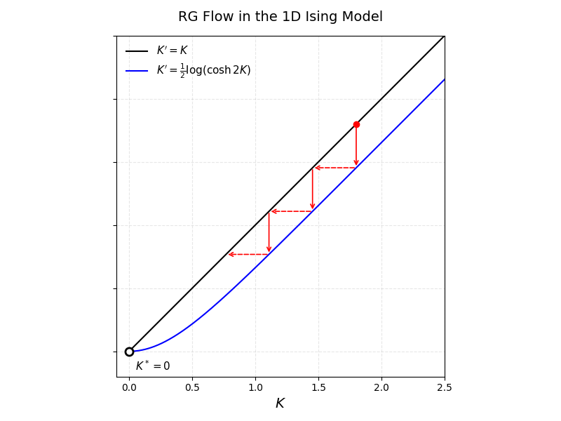
But ultimately, what we’re most interested in is not what happens when we coarse-grain once, but an infinite number of times. If you imagine our coarse-graining procedure as defining a trajectory in the space of couplings (called the renormalization group flow), then what we want to find are the fixed points of this flow.

Let $K’(K)$ denote the value of the coupling constant $K’$ that results from one iteration of our RG flow starting from the coupling constant $K$. Fixed points of our renormalization group flow correspond to values of $K$ where $K’ = K$. The 1D Ising model has two fixed points: $K = 0$ and $K = \infty$.

For $K=0$, we have that:

\[\begin{align} K'(0) &= \frac{1}{2} \log \left(\frac{e^{2K} + e^{-2K}}{2}\right) \\ &= \frac{1}{2} \log \left(1 \right) \\ &= 0 \end{align}\]

And for $K = \infty$, we have that:

\[\begin{align} K'(\infty) &= \lim_{K \rightarrow \infty} \frac{1}{2} \log \left(\frac{e^{2K} + e^{-2K}}{2}\right) \\ &= \frac{1}{2} \log \infty \\ &= \infty \end{align}\]

These two fixed points make physical sense. The $K=0$ fixed point corresponds to the disordered phase: there is no interaction between neighboring lattice sites, so they fluctuate independently. If you only retain every other lattice site, then the new lattice will still have independent sites. The $K = \infty$ fixed point corresponds to the ordered phase: there is an infinite energetic cost to any two neighboring spins being anti-aligned, so the whole lattice will point in the same direction. If you retain only the even sites, they will still all point in the same direction.

But we don’t just care about the existence of fixed points—we also care about the behavior of the RG flow in the neighborhood of each fixed point. If your system is close in coupling space to a fixed point and you coarse-grain, will it eventually flow toward the fixed point (stable) or away from it (unstable)?

For there to be a phase transition, we would need a critical value $K_c$ such that for all values $K < K_c$, the system flows to the $K = 0$ fixed point (disordered phase), and for all values $K > K_c$, the system flows to the $K = \infty$ fixed point (ordered phase). This critical value would mark the boundary between two distinct phases.

However, the 1D Ising model has no phase transition. To demonstrate this, we can show that for any finite value of $K$, the RG flow eventually leads to the $K = 0$ fixed point. Only the $K = \infty$ point itself remains at $K = \infty$. This means there’s no finite critical temperature separating distinct phases—the system is always disordered at any finite coupling strength.

Taking $K \ll 1$, we can show that:

\[\begin{align} K'(K) &=\frac{1}{2} \log \left (\frac{e^{2K} + e^{-2K}}{2} \right) \\ &\approx \frac{1}{2} \log \left (1 + 2 K^2 \right) \\ &\approx K^2 \end{align}\]

We assumed $K$ to be small, so $K’ \sim \Theta(K^2)$ is even smaller. It follows that for small values of $K$, the fixed point of the RG flow is the $K = 0$ fixed point.

For large $K$, we have that:

\[\begin{align} K'(K) &= \frac{1}{2} \log \left ( \frac{e^{2K} + e^{-2K}}{2} \right ) \\ &\le \frac{1}{2} \log \left ( \frac{e^{2K}}{2}\right) \\ &= K - \frac{\ln 2}{2} \\ \end{align}\]

So for large $K$, we have that $K’ < K$.

This is an indication that the only stable fixed point is $K^{*} = 0$—the disordered phase. We have no phase transition for the 1D Ising model.