How to Find the PDF of a Function of Random Variable

Let $X$ be a random variable with a probability density function (PDF) given by \(f(x)\) and a cumulative distribution function (CDF) given by \(F(x)\). Let $Y$ be a random variable such that $h(X) = Y$. Let $g(y)$ and $G(y)$ be the PDF and CDF of $Y$, respectively.

The question is: given the PDF and CDF of $X$, how does one find the PDF and CDF of $Y$?

This is a ridiculously simple question. When I was first learning probability theory, it was the very first question I had. Yet, somewhat frustratingly, the usual sources of information (e.g Wikipedia) don’t lay out the procedure simply and in full generality. It was only until I read Gavin Crooks’ Field Guide To Probability Distributions that I found what I was looking for. It’s quite simple though. Here’s how it works.

The short explanation is that the relationship between the two random variables is most naturally expressed through their CDFs. Specifically, the relation is $G(y) = F(h^{-1}(y))$. Here’s the derivation:

\[\begin{align} G(y) &= P(Y \le y) \\ &= P(h^{-1}(Y) \le h^{-1}(y)) \\ &= P(X \le h^{-1}(y)) \\ &= F(h^{-1}(y)) \end{align}\]

The key is to recall the definition of the CDF as the probability of the random variable being less than or equal to a specific value. In the step where we apply $h^{-1}$ to both sides of the inequality, we are implicitly assuming that $h$ is monotonic (which, when combined with continuity, implies that $h$ is a bijection between its domain and range). Though it isn’t too difficult to generalize to the case when $h$ isn’t a bijection.

Once we have the relationship between the CDFs, we can find the relationship between the PDFs using the chain rule.

\[g(y) = \frac{d}{dy} G(y) = \frac{d}{dy} F(h^{-1}(y)) = f(h^{-1}(y)) \left|\frac{dx}{dy}\right|\]

So the PDF of $Y$ is given the by PDF of $X$ evaluated at the corresponding point in the domain multiplied by the derivative of the inverse function. This scaling factor is called the Jacobian and appears all over the place in more advanced applications of multivariable calculus, especially in differential geometry. In this example, we are working with single variables, so the best linear approximation of a function is given by the derivative. When dealing with joint probability distributions, we will extend this concept to multivariable transformations. The best linear approximation to a function between multiple variables is given by a matrix that sends small perturbations in the inputs to small perturbations in the outputs. The Jacobian is the determinant of this matrix and gives the local scaling factor when going from the domain to the corresponding point in the codomain.

In discussions about functions of random variables, they often start with the explanation in terms of Jacobians and local scaling factors. This is probably the more “sophisticated” perspective, but I like the derivation that starts with CDFs as the math is simpler and easier to follow. But it’s useful to be able to think about functions of random variables both in terms of the relationship between the CDFs and in terms of the relationship between the PDFs.

Another way to think about the PDF of a function of a random variable is as a type of expectation value. Loosely, it would be “what is the chance that for a given output value $y$, a randomly chosen value $x$ is one which is mapped to $y$ by $h$?”. It’s given by the following equation:

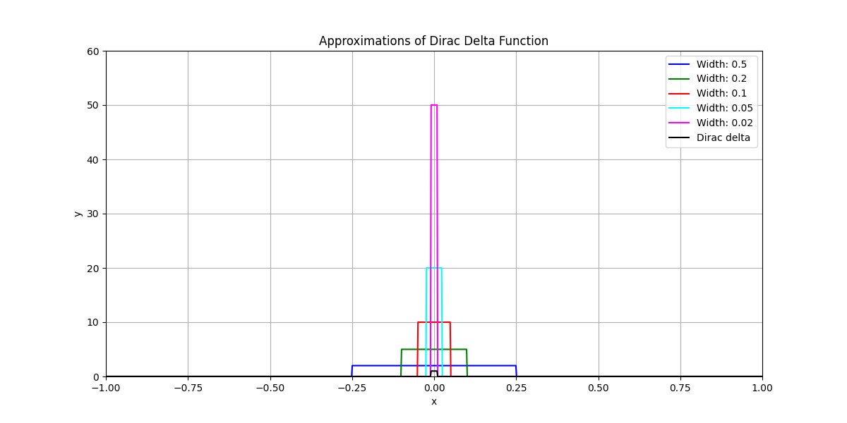
\[g(y) = \int dx f(x) \delta(h(x) - y)\]

We can show that this formulation for the PDF of $Y$ is equivalent to the previous formulation in terms of the Jacobian. First, we will need to review some facts about the Dirac delta function. One important property of the Dirac delta function is that scaling its argument results in an inverse scaling of the function itself. This property can be expressed mathematically as:

\[\delta(ax) = \frac{1}{|a|} \delta(x)\]

This can be most easily seen by considering the Dirac delta function as the limit of some sequence of narrower and narrower distributions. If before passing to the limit, we scale each of the distributions in our sequence by $a$, we can demonstrate the desired result.

Next, we notice that if $x_0$ is a root of some function $h$, then by Taylor expansion we have that near $x_0$:

\[h(x) \approx h(x_0) + h'(x_0)(x - x_0) = h'(x_0)(x - x_0)\]

The Dirac delta function is only non-zero when its argument is zero, so we’re particularly interested in the behavior of $h(x)$ near its roots. Using this linear approximation and the scaling property of the Dirac delta function, we can write:

\[\delta(h(x)) \approx \delta(h'(x_0)(x - x_0)) = \frac{1}{\lvert h'(x_0)\rvert} \delta(x - x_0)\]

The $\frac{1}{\lvert h’(x_0)\rvert}$ in front of the Dirac delta should look familiar. The inverse function theorem tells us that the value of the derivative of the inverse function at a given point in the codomain is equal to the reciprocal of the value of the derivative evaluated at the corresponding point in the domain. Recalling that $Y = h(X)$ and letting $x_0 = h^{-1}(y)$, we then have that

\[\begin{align} g(y) &= \int dx f(x) \delta(h(x) - y) \\ &= \int dx f(x) \delta(h'(x_0)(x-x_0)) \\ &= \int dx f(x) \frac{1}{|h'(x_0)|} \delta(x-x_0) \\ &= f(x_0) \frac{1}{|h'(x_0)|} \\ &= f(h^{-1}(y)) \left | \frac{dx}{dy} \right | \end{align}\]

There is yet another perspective on this formula. The multivariable function

\[u(x,y) = f(x) \delta(h(x) -y)\]

is precisely the joint distribution of $X$ and $Y$. However, due to the presence of the Dirac delta function, this distribution is singular and concentrates all its probability mass on a one-dimensional manifold within the two-dimensional $(x,y)$ space. This follows from the fact that $Y$ is a deterministic function of $X$; the intrinsic dimensionality of the probability space shouldn’t increase by appending $Y$ to our distribution. When we are integrating $u$ with respect to $x$, we are marginalizing with respect to $x$, leaving us only the PDF for $Y$.

(This idea—starting with a random variable, artificially constructing a joint distribution by adding a deterministic function of that variable, then marginalizing over the original variable—is surprisingly ubiquitous in physics.)

Let’s derive the PDF of some example distributions to show how it works.

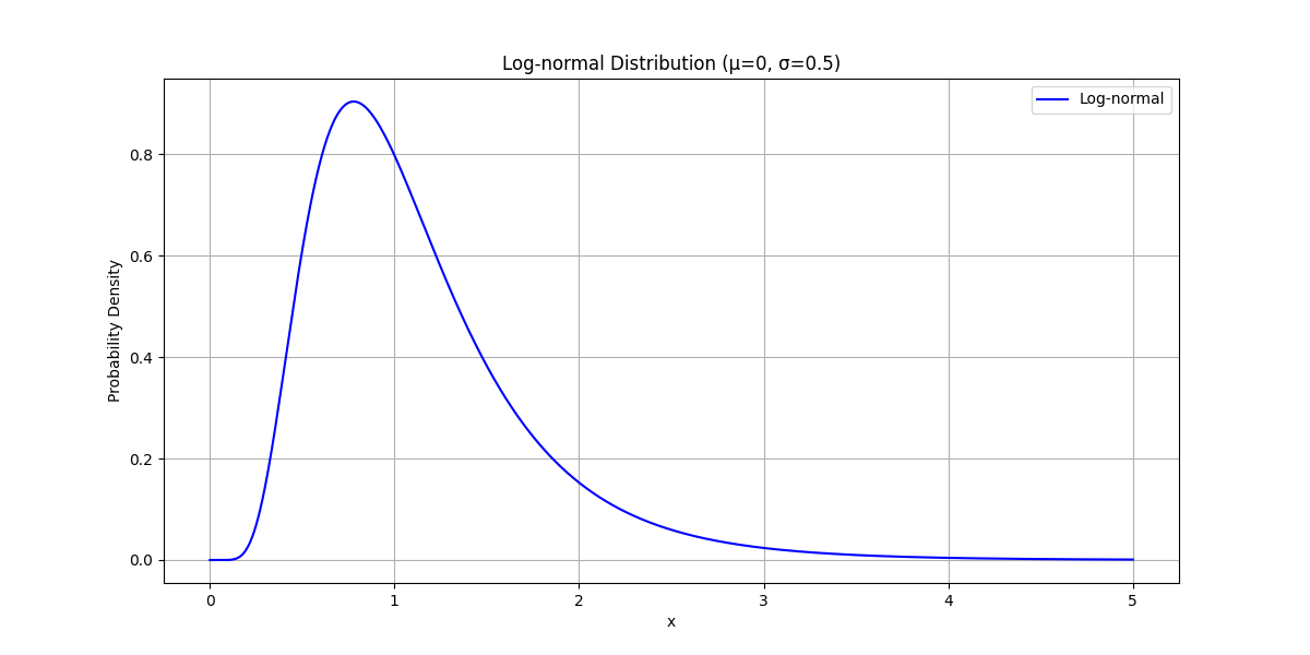
The log-normal distribution

The log-normal distribution describes any random quantity whose order-of-magnitude is normally-distributed. It’s a fat-tailed distribution defined over $(0, \infty)$ which can obtained by exponentiating a normally-distributed random variable.

\[Y = h(X) = e^X\]

where $Y$ is a log-normal-distributed random variable and $X$ is a normally-distributed random variable. We then have for the CDF of $Y$:

\[G(Y) = F(h^{-1}(y)) = F(\log(y)) = \text{erf}(\log(y))\]

Then we take the derivative to get that

$g(y) = \frac{1}{y} \frac{1}{\sqrt{2 \pi \sigma^2}} e^{- \frac{(\log y - \mu)^2}{2 \sigma^2}}$

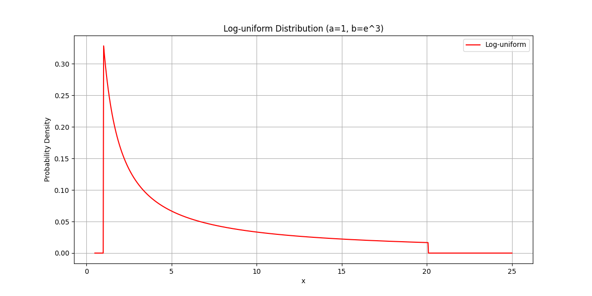
The log-uniform distribution

The log-uniform distribution describes a random quantity whose order-of-magnitude is uniformally-distributed. Similar to the log-normal distribution, the log-uniform distribution can be obtained by exponentiating a uniformally-distributed random variable. If $[a,b]$ is the support of $X$, the uniformally-distributed random variable, then the support of $Y$ is $[e^a, e^b]$. For the CDF of $Y$, we have:

\[G(y) = \log(y)\]

And for the PDF, we have:

\[g(y) = \frac{1}{y}\]

The log-uniform distribution is also called the reciprocal distribution due to the functional form of its PDF.