Inverse Transform Sampling Explained
Consider the easiest sampling problem: sampling from a univariate distribution where we have an analytical expression for the probability density function $g$ (including the normalization constant). How does one practically go about sampling from $g$? As in, what is a set of instructions that you can give a computer such that are confident that the the produced number will be drawn from the intended distribution?
One technique is inverse transform sampling (which is a terrible, nondescriptive name—but whatever). Inverse transform sampling relies on three facts:
-
We know how to simulate uniform random variables $X \sim \mathcal{U}(0,1)$ on a computer.
-
We know how functions of random variables work.
-
We know how to compute the values of functions on a computer.
How do you simulate a uniform random variable on a computer? You use a pseudorandom number generator. These are deterministic algorithms which produce values that might as well be random (often you do need to supply an initial random seed). I honestly don’t remember the precise details for how the most popular pseudorandom number generators work. (I think the algorithms involve large prime numbers and modular arithmetic?). But let’s just take it on faith that the problem of sampling from the uniform distribution on $[0,1]$ is solved.
How do we go from sampling the uniform random variable $X \sim \mathcal{U}(0,1)$ to sampling from the desired random variable $Y \sim g$?
In my previous post on how to find the PDF of a function of random variable, we showed that if $F$ is the cumulative distribution function (CDF) of $X$, $G$ is the CDF of Y, and $h$ is a function such that $h(X) = Y$, then we have that
\[G(y) = F(h^{-1}(y))\]In the original post, we were given the function $h$ and the original CDF $F$, and we were tasked with finding the target CDF $G$. Our current problem is a little different. Here, we have both the original CDF $F$ and target CDF $G$, but we are trying to find what function $h$ allows us go from $F$ to $G$. Using the fact that $h(x) = y$, we can rewrite the above equation in a more useful form:
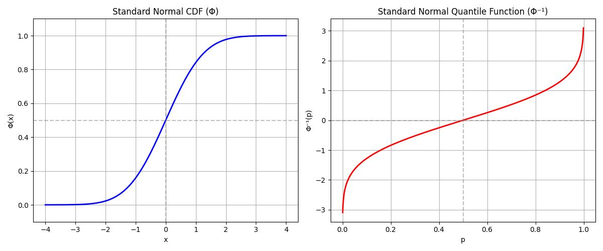
\[h(x) = G^{-1}(F(x))\]So $h$ turns out to be the composition of two functions: $F$, the CDF of our uniform random variable, and $G$, the inverse of the CDF of our target distribution. The inverse of the cumulative distribution function actually has a name: the quantile function. If the cumulative distribution takes values in the sample space of the random variable and maps it to probabilities (the probability that the attained value of the random variable will be less than or equal to the inputted value), then the quantile function takes probabilities and maps them to values in the sample space.

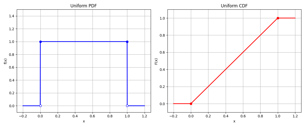
It turns out that finding $F$ is easy. The uniform random variable has a probability density function of the form
\[f(x) = \begin{cases} 0 & \text{if } x < 0 \\ 1 & \text{if } 0 < x < 1 \\ 0 & \text{if } x > 1 \end{cases}\]To find $F$, we just take the antiderivative of $f$. Setting the constant $C$ such that $F(0) = 0$, we have that
\[F(x) = \begin{cases} 0 & \text{if } x < 0 \\ x & \text{if } 0 ≤ x ≤ 1 \\ 1 & \text{if } x > 1 \end{cases}\]
We have that on the support of $f$ (the interval $[0,1]$), $F(x) = x$! So in fact our equation for $h$ reduces down to:
\[h(x) = G^{-1}(x)\]So to go from a uniform random variable $X$ to any desired distribution $Y \sim g$, you just have to apply the quantile function $G^{-1}$ of the desired distribution to $X$.
(I believe the reason why this technique is called “inverse transform sampling” is that the required function is the inverse of the cumulative distribution function. If I were to rename the technique, I would call it “quantile sampling”.)
This is great! With inverse transform sampling, we’ve reduced the computational task of sampling from a distribution to the computational task of computing its quantile function $G^{-1}$.
Let’s work through a quick example.
The Exponential Distribution
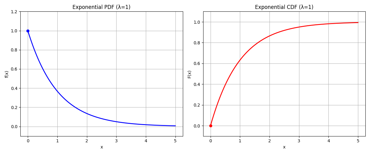
An exponential distribution with rate parameter $\lambda$ has a PDF of the form:
\[g(y) = \lambda e^{-\lambda y}\]The CDF is then:
\[G(y) = 1 - e^{-\lambda y}\]
To find $G^{-1}$, we let $x$ = $G(y)$ and then isolate $x$ in the above equation.
\[x = 1 - e^{-\lambda y} \longrightarrow y = - \frac{1}{\lambda} \ln (1 - x)\]Recall that we will be applying our function to $X$, a uniform random variable on $[0,1]$. If $X$ is a uniform random variable on $[0,1]$, then $1 - X$ is also a uniform random variable on $[0,1]$. So we are free to replace the $1-x$ in the logarithm with just $x$. So if $X$ is a uniform random variable and $Y$ is an exponential random variable with rate parameter $\lambda$, we have that:
\[Y = \frac{1}{\lambda} \ln \frac{1}{X}\]