Location, Scale, and Power
For any given parametric family of probability distributions, there are many different ways that you can parametrize it. For example, for the normal distribution, you can parametrize it by:
- Using the mean $\mu$ and the standard deviation $\sigma$
- Using the mean $\mu$ and the variance $\sigma^2$
- Using the mean $\mu$ and the second moment $\mu^2 + \sigma^2$
Going between the most common parametrizations of the normal distribution is pretty straightforward, so we rarely focus too much on which specific parameterization that we are using.
But in general, there are certain types of parameters that appear over and over again with different parametric families. For example, there are support parameters which define the domain in which the probability distribution is non-zero. The parametric family of uniform distributions on $\mathbb{R}$ can be parametrized by $\mathbf{U}(x; a, b)$ where $a$ and $b$ are the left and right end-points of the interval of support, respectively. Degrees of freedom parameters appear in distributions like the chi-squared and F-distributions, which are commonly used in statistical hypothesis testing. The ‘degrees of freedom’ typically correspond to the size of the data set sampled from the underlying population. Different-sized data sets lead to different distributions for various statistics (e.g., the distribution of the sum of squared residuals).
I want to focus on three types of parameters: location, scale, and power parameters. These parameters are not only ubiquitous in parametric families of probability distributions, but they are also notable for their distinct interactions with algebraic operations on random variables.
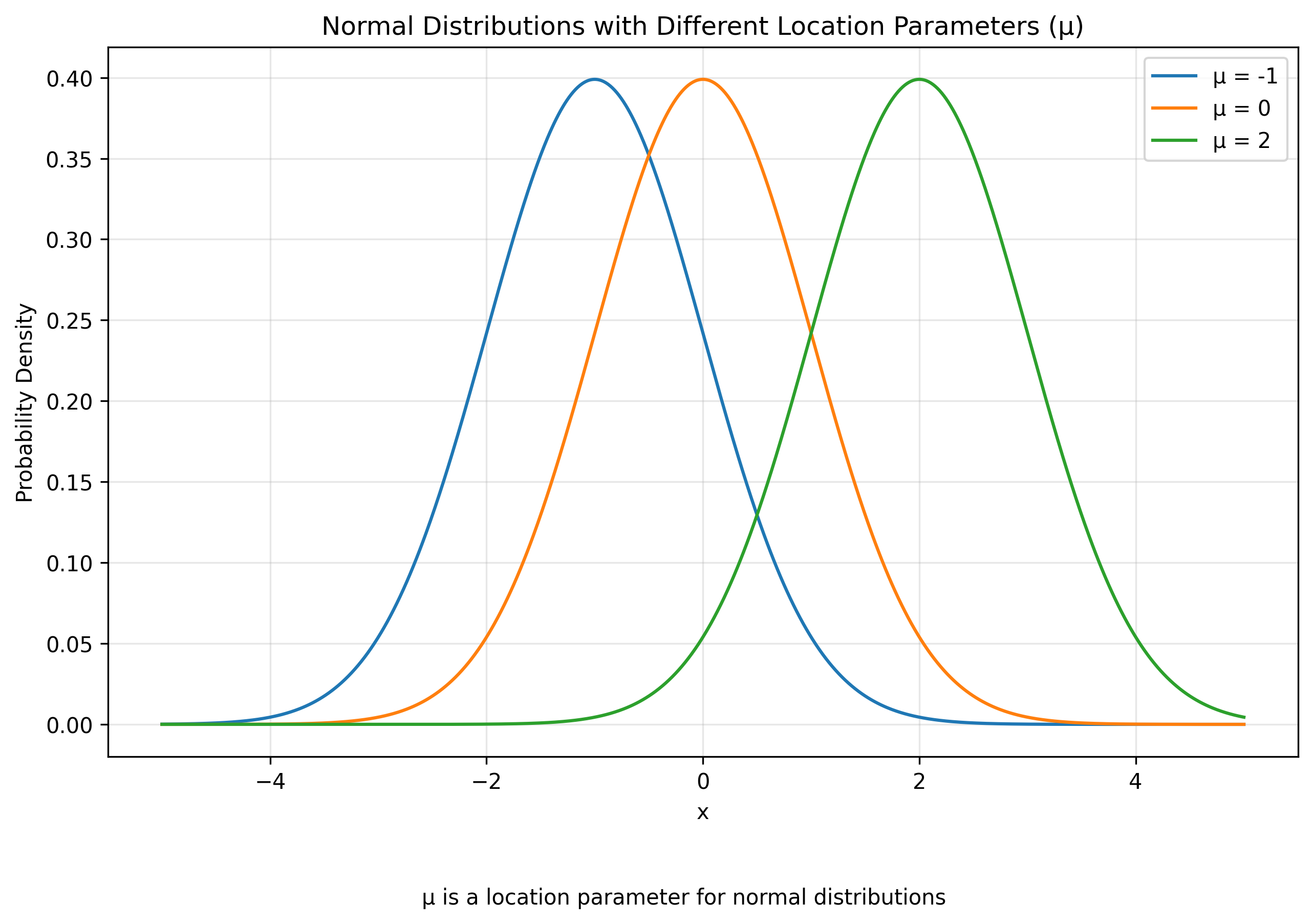
A location parameter is exactly what it sounds like: a parameter that tells you where a probability distribution in the parametric family is located. Consider the alternative parametrization of the uniform distribution $\mathbf{U}(x; s, a)$. Here, we have that $s$ is the center of the interval and $a$ is the width of the interval. So if $s=3$ and $a=4$, you would have the uniform distribution on the interval $[1,5]$.
Let $X \sim \mathbf{U}(x; s, a)$. Then if you add a number $b$ to $X$, you will define a new random variable $Y$ which is shifted by $b$ to the right.
\[Y = b + X\]This new random variable will also be a uniform distribution—one whose location parameter is $s + b$. This is the defining property of location parameters: the addition of a number to a random variable in the parametric family is equivalent to adding the same number to the value of the location parameter. Let $\mathbf{P}(x; s)$ be a generic one-parameter family of probability distributions with location parameter $s$. Then we have that:
\[b + \mathbf{P}(x; s) = \mathbf{P}(x; s + b)\]Location parameters are the most common type of parameter. In most parametric families, convention dictates that the value of the location parameter equals the mean of the probability distribution. Location parameters are common in probability distributions defined on the entire real line or those with compact support. However, they are less common for distributions that lie on the infinite half-interval $(0, \infty)$. Distributions on the infinite half-interval (e.g., the exponential distribution) usually have some physical interpretation that makes zero special, breaking the implicit translation invariance typical of parametric families featuring a location parameter.
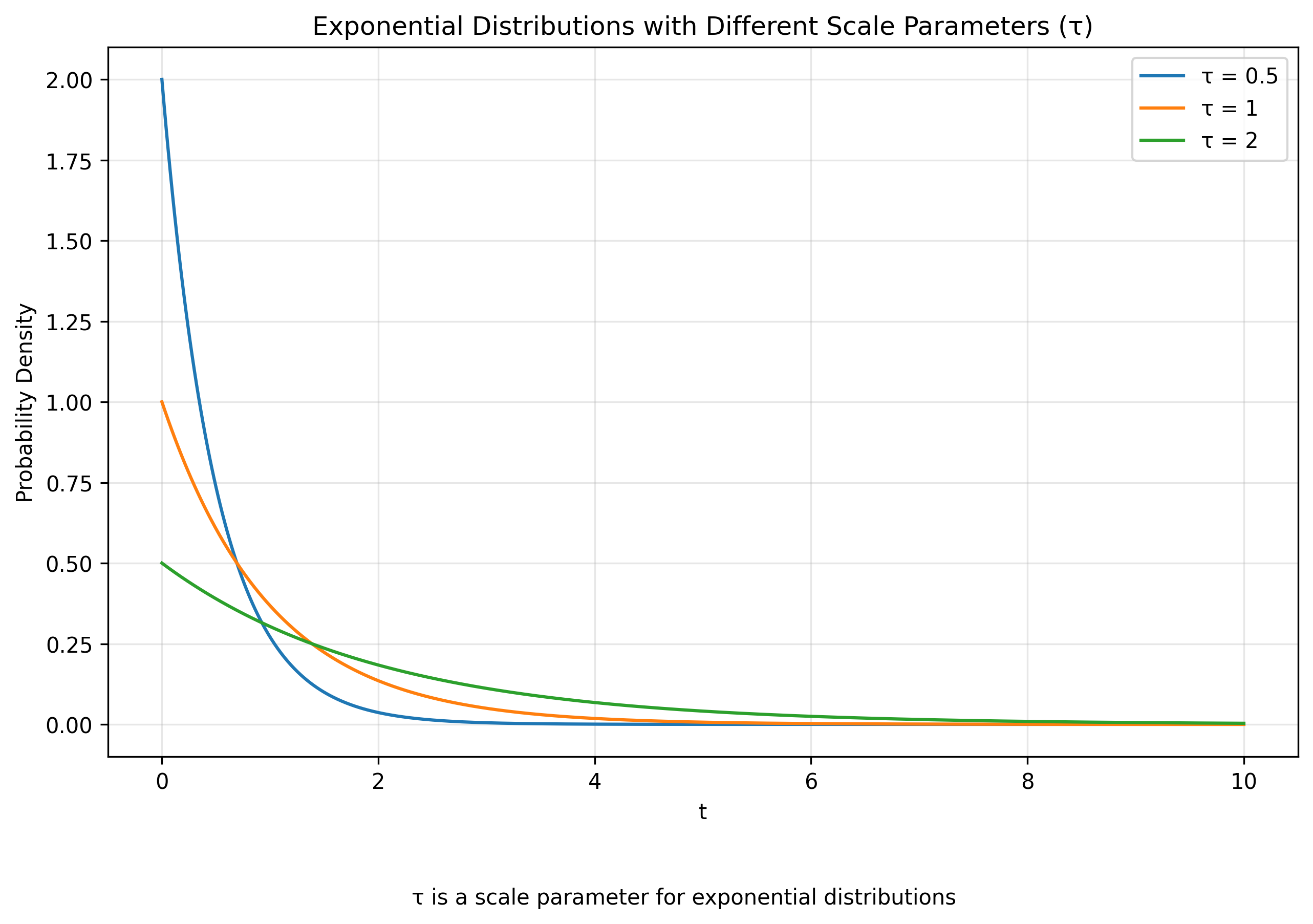
However, one type of parameter features prominently in parametric families whose domain is the infinite half-interval: scale parameters. A scale parameter governs the ‘spread’ of the probability distribution: a large value of the scale parameter corresponds to a more spread-out distribution, while a small value corresponds to a more concentrated one. This is an active interpretation of the scale parameter. Alternatively, one could take a passive interpretation where the actual physical quantity remains unchanged, but our perception of it changes. This perceptual change can be visualized as a ‘zooming process’ where large scale parameters correspond to zooming in and small values to zooming out. Or it could be thought of as changing the units of measurement, where ‘smaller’ units (like inches) correspond to large values of the scale parameter and ‘larger’ units (like miles) correspond to small values.
Let’s revisit our old friend the parametric family of uniform distributions and consider only those distributions that are centered at the origin: $\mathbf{T}(x; a) = \mathbf{U}(x; 0, a)$. Given a scale parameter value of $a$, the support of the distribution is $[\frac{-a}{2}, \frac{a}{2}]$. If we multiply a member of $\mathbf{T}$ by a number $b$, then the new random variable will be a uniform distribution centered at the origin whose support is scaled by $b$.
\[b * \mathbf{T}(x; a) =\mathbf{T}(x; a b)\]While location parameters are closely associated with the mean of the probability distribution, scale parameters have more diverse interpretations. With the case of the exponential distribution
\[\mathbf{E}(t; \tau) = \frac{1}{\tau} e^{-\frac{t}{\tau}}\]the parameter $\tau$ is a scale parameter that is equal to the mean of the distribution. But in the case of the normal distribution centered at the origin, when parametrized by the standard deviation $\sigma$, $\sigma$ functions as a scale parameter. $\sigma$ is not associated with the mean of the distribution, but the variance (specifically, $\sigma$ is the square root of the variance).
Location and scale parameters can actually be related by exponentiation of random variables. Let $\mathbf{P}(x; \mu)$ and $\mathbf{Q}(x; a)$ be two parametric families related by the equation:
\[\mathbf{Q}(x; a) = \text{exp} \left [\mathbf{P}(x; \mu) \right ]\]If we have that $\mu$ is a location parameter, then $a$ is a scale parameter with $a = e^\mu$. This connection between location and scale parameters shouldn’t be too surprising. Exponentiation is the unique continuous map from the real numbers as an additive group to the positive real numbers as a multiplicative group. (I believe this intuition is also behind the relationship between Lie Algebra and Lie Groups: why vector addition of matrices gets mapped to group multiplication of matrices). Location parameters and scale parameters are in some sense the parametric manifestation of addition and multiplication, respectively.
We might naturally wonder: what happens when we exponentiate a random variable with a scale parameter? This leads us to a third important type: power parameters.
To understand power parameters, consider a random variable $X$ that has a scale parameter $\sigma$. We know that for any constant $k$, $kX$ has the same distribution as $X$ with scale parameter $k\sigma$. Now let’s consider $Y = \exp(X)$. What happens when we raise $Y$ to a power $k$?
\[Y^k = (\exp(X))^k = \exp(kX)\]We can see that raising $Y$ to the $k$th power corresponds to multiplying $X$ by $k$. In other words, power operations on $Y$ translate to scale operations on $X$. This relationship motivates the definition of a power parameter. A power parameter $\beta$ is one that interacts with power operations in a way analogous to how scale parameters interact with multiplication.
Power parameters are not as common as location and scale parameters, but they fit a similar theme where they are defined by a key algebraic relationship. Let $\mathbf{P}(x; \beta)$ be a one-parameter family with power parameter $\beta$. The defining relationship for power parameters is
\[[\mathbf{P}(x; \beta)]^{1/k} = \mathbf{P}(x; \beta k)\](Why are we defining power parameters such that raising to the $1/k$ power causes the power parameter to be multiplied by $k$? It’s because whatever you do to a random variable, the opposite happens to the argument of the cumulative distribution function. So raising the random variable to the $1/k$ power causes the argument of the cumulative distribution to be raised to the $k$ power—which then trickles down to the probability density function as well. This convention ends up being a more natural and helpful way to think about power parameters.)
Power parameters are useful for augmenting parametric families to include a wider class of distributions. For example, consider the exponential family $\mathbf{E}$. This is a one-parameter family. We can consider the two-parameter family of distributions defined by
\[\mathbf{W}(t; \tau, \beta) = \left [\mathbf{E} \left (\frac{t}{\tau}; 1 \right) \right]^{\frac{1}{\beta}}\](The reason for the particularity of the definition is that it’s required that $\frac{t}{\tau}$ get raised to the given power, not just $t$ individually. I’m not sure if there is a more elegant way to represent that distinction using the notation that I decided to adopt.)
This family of distributions is called the Weibull distribution. And since we know how to find the PDFs of functions of random variables, we can quickly derive the PDF of the Weibull distribution.
\[\mathbf{W}(t; \tau, \beta) = \frac{\beta}{\tau} \left( \frac{t}{\tau}\right)^{\beta - 1} e^{-(t/\tau)^\beta}\]