The Mean-Field Theory of Two-Layer Neural Networks

A two-layer neural network is a sum of $N$ simple units:

\[f(x; \theta) = \sum_{i=1}^{N} v_i \, \sigma(w_i \cdot x).\]

Each unit—each neuron—does three things:

1. Projects the input $x$ onto a direction $w_i$
2. Applies a scalar nonlinearity $\sigma$
3. Contributes to the output with weight $v_i$

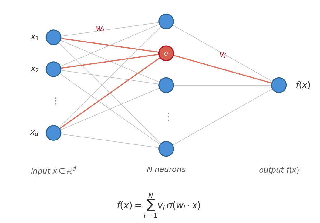
A “feature” is a relevant aspect of the input distribution. If the directions $w_i$ were fixed in advance, this would be linear regression on a fixed set of features—the model would be linear in its trainable parameters (the second-layer weights). But in a two-layer network, the first-layer weights are trained too. Two-layer neural networks then differ from linearly-parametrized networks in that they can learn the relevant features. A model that learns its own features is necessarily a nonlinear function of its parameters—which makes the loss landscape non-convex.

\[L(\theta) = \mathbb{E}_{x}\left[\left(f(x; \theta) - f^*(x)\right)^2\right],\]

where $f^\ast$ is the target function and $L$ is the loss function.

To train the model, we must perform some variant of gradient descent on the loss function. But how do we know that gradient descent will work—that the iterates will converge to a global minimum of the loss? It’s hard to prove things in the non-convex setting. Gradient descent on a generic non-convex landscape can get trapped at a local minimum. Yet everyday experience with deep learning suggests the opposite: make the network wide enough, and gradient descent drives the training loss to near-zero reliably. At the beginning of the deep learning revolution, this simple fact had no adequate explanation in theory—not even for the two-layer network, the simplest network that learns features at all.

In the spring of 2018, an explanation arrived. Over the course of five weeks, four different groups posted arXiv papers describing the dynamics of two-layer neural networks in the mean-field regime—the limit as the width of the network goes to infinity. They all shared a common insight: instead of tracking the long vector of parameters, it’s better to track the empirical distribution over neurons.

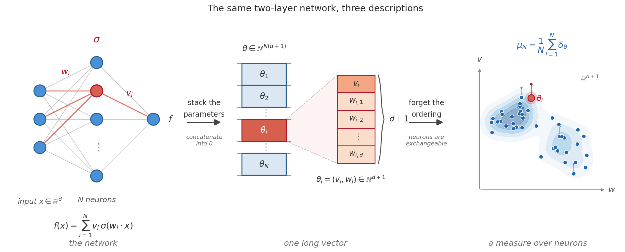
All four groups answered the question: in the infinite-width limit, do the dynamics of gradient descent converge to a distributional description? Three of the groups tackled the slightly harder question: do those dynamics provably reach a global minimum of the loss?

• Mei, Montanari, and Nguyen (April 2018) wanted to answer whether stochastic gradient descent (SGD) converges to a global optimum of the loss function. In their setting, they showed that the distribution of neurons evolves according to a nonlinear partial differential equation—which they called distribution dynamics. Using this description, they were then able to provide a global convergence guarantee for noisy SGD.

• Rotskoff and Vanden-Eijnden (May 2018) reinterpreted SGD as an interacting particle system in which each neuron corresponds to a particle and the loss function corresponds to the potential. They were able to show that the probability distribution of the neurons evolves according to a nonlinear Liouville equation. Using the law of large numbers, they showed that the empirical distribution at initialization converges to a well-defined distribution, which can then be used to show weak convergence for the entire trajectory of measures. From this, they were able to prove convergence to a global optimum of the loss.

• Sirignano and Spiliopoulos (May 2018) investigated the training dynamics of SGD in the limit where both the width of the network and the number of iterations go to infinity. They proved that the dynamics converge to a nonlinear partial differential equation. They also showed that in the infinite-width limit, the neurons asymptotically become independent from each other—a property known as propagation of chaos.

• Chizat and Bach (May 2018) identified the evolution of the measure as a Wasserstein gradient flow: a gradient flow in the space of probability measures endowed with the Wasserstein metric. They showed that this flow converges to a global minimizer of the unregularized loss.

Collectively, they founded what is now called the mean-field theory of two-layer neural networks.

(“Mean field” is unfortunately one of the most overloaded phrases in applied mathematics. In this article, the term refers to the McKean–Vlasov-type limit of two-layer neural network training dynamics. This is not to be confused with dynamical mean-field theory which tracks order parameters like kernels and correlation functions rather than a particle density. Nor is it to be confused with mean-field variational inference in Bayesian machine learning which refers to product-measure approximations.)

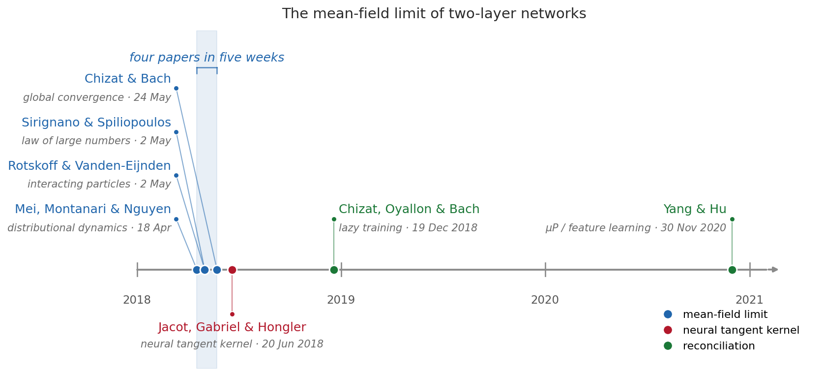
However, that wasn’t the end of the infinite-width story. One month later, a fifth paper landed. Jacot, Gabriel, and Hongler (June 2018) also studied neural networks in the infinite-width limit, and also concluded that gradient descent provably fits the training data. But their description looked nothing like the mean-field picture. In their limit, the network behaves as a kernel method—a linear model built on a fixed set of features—with the kernel being the neural tangent kernel.

So we have two incompatible pictures of what training looks like in the infinite-width limit. Which one describes the real-world networks we actually train?

Resolving that question fell to Chizat, Oyallon, and Bach (December 2018). They identified two regimes: the lazy regime, in which the parameters barely move from their initialization, and the feature-learning regime, in which the parameters move an $O(1)$ distance from their initialization.

Which regime the network operates in depends on how the output is scaled. The NTK scaling puts you in the lazy regime, while the mean-field scaling puts you in the feature-learning regime. And it is ultimately the feature-learning regime that more accurately models neural network training dynamics.

Yang and Hu (2020) later recovered this dichotomy as a complete classification. They proved that, in the infinite-width limit, every well-behaved parametrization either admits feature learning or is equivalent to a kernel method. Within the feature-learning class, they identified a special parametrization: the maximal update parametrization ($\mu P$). With $\mu P$, every layer learns features at the largest rate possible while remaining stable.

Mean-Field Parametrization

We will walk through the derivation of the mean-field dynamics of two-layer neural networks. We will follow most closely the approach of Chizat and Bach, though we will note the other three perspectives where appropriate.

First, we set up the two-layer neural network. The network is composed of $N$ individual units called neurons. Each neuron has its own parameters and can be viewed as a function of the input: it projects the input down, composes with a nonlinearity, and then weights the result. Bundling everything the $i$-th neuron owns into a single vector $\theta_i = (v_i, w_i) \in \mathbb{R}^{d+1}$, we write the single-neuron function as

\[g(x; \theta_i) = v_i \, \sigma(w_i \cdot x).\]

We can then define the network in the mean-field parametrization, which averages the neuron outputs instead of simply summing them:

\[f(x; \theta_1, \ldots, \theta_N) = \frac{1}{N} \sum_{i=1}^{N} g(x; \theta_i)\]

Notice that $f$ has a particular symmetry. If you relabel the neurons—for example, swapping $\theta_3$ with $\theta_{15}$—the value of the function remains unchanged. The network exhibits an exchange symmetry with respect to the neurons. Consequently, what matters for the output isn’t the ordered list of neuron values, but the unordered set of those values. The information in the unordered set can be carried by an empirical measure that places an atom at each location corresponding to the value of a neuron.

\[\mu_N = \frac{1}{N} \sum_{i=1}^{N} \delta_{\theta_i},\]

The network output is then an integral of the single-neuron function against this measure:

\[f(x; \mu_N) = \int g(x; \theta) \, d\mu_N(\theta)\]

In physics jargon, we can say that the neurons represent identical particles. Particles in the real world are identical as well. For example, there’s no way to tell two hydrogen atoms apart. Every property—the mass, the charge—is the same for every hydrogen atom. And when working with identical particles, it doesn’t make sense to have a description that implicitly tells them apart by giving them a label. With the empirical measure, we only encode the spatial density of the neurons in parameter space—the only physically meaningful information.

Consider the population mean-squared error loss:

\[L_N(\theta_1, \ldots, \theta_N) = \frac{1}{2} \, \mathbb{E}_{(x,y)} \big[ (f(x; \theta_1, \ldots, \theta_N) - y)^2 \big]\]

We want to re-express the loss in terms of the measure. We can do because $f$ depends on the parameters only through $\mu_N$.

\[\mathcal{L}[\mu] = \frac{1}{2} \mathbb{E}_{(x,y)} \left[ \left( \int g(x; \theta) \, d\mu(\theta) - y \right)^{2} \right]\]

The loss function has been promoted to a loss functional, defined on the space of probability measures. And notice that the functional is well-defined for any probability measure $\mu$ over $\mathbb{R}^{d+1}$, not just empirical measures supported on $N$ points.

We can now explain the terminology “mean-field”. It’s jargon from statistical physics. We can describe a system as mean-field when every particle responds only to the aggregate field generated by the other particles. The mean-field description applies here precisely because the output $f$ can be expressed as an expectation with respect to the empirical measure—which is made possible by the $1/N$ pre-factor that defines the mean-field parametrization.

It’s useful to break down the loss functional into separate terms. Expanding the square in $\mathcal{L}$:

\[\mathcal{L}[\mu] = \frac{1}{2} \, \mathbb{E}\!\left[y^2\right] + \int V(\theta) \, d\mu(\theta) + \frac{1}{2} \iint U(\theta, \theta') \, d\mu(\theta) \, d\mu(\theta')\]

where

\[V(\theta) = -\mathbb{E}_{(x,y)} \big[ y \, g(x; \theta) \big], \qquad U(\theta, \theta') = \mathbb{E}_{x} \big[ g(x; \theta) \, g(x; \theta') \big]\]

There are three terms: a constant term, a single-particle potential, and an interacting-particle potential. The single-particle potential $V$ pulls each neuron toward configurations whose output correlates with the labels. The interaction $U$ raises the energy of pairs of neurons whose outputs are positively correlated, causing a repulsion force between neurons.

Wasserstein Gradient Flow

It’s time to tackle the dynamics. What does gradient descent on the $N$ neurons correspond to in terms of the dynamics of $\mu_N$? Since measures are unfamiliar territory, we first need to introduce some mathematical machinery.

Given a loss functional $\mathcal{L}$, the first variation $\frac{\delta \mathcal{L}}{\delta \mu}$ tells you how small density perturbations of the measure change the value of the functional: perturb $\mu$ by a small signed measure $\varepsilon \chi$, and the loss changes, to first order, by $\varepsilon \int \frac{\delta \mathcal{L}}{\delta \mu} \, d\chi$. For our MSE loss, it is straightforward to compute the first variation:

\[\frac{\delta \mathcal{L}}{\delta \mu}(\theta) = \mathbb{E}_{(x,y)} \big[ \left( f(x; \mu) - y \right) g(x; \theta) \big]\]

This makes sense: the first variation at $\theta$ is the marginal cost of adding neuron-mass at the location $\theta$. It is large and positive at locations where the neuron fires in phase with the current residual $f(x;\mu) - y$, so adding mass there would only increase the loss. It is negative at locations where the neuron fires out of phase with the residual.

To decrease the loss, you need to move neuron-mass from locations with higher values of the first variation to locations with lower values. However, because gradient descent only nudges the parameters, the corresponding particle description must also exhibit local dynamics. The neurons aren’t allowed to teleport in order to minimize the loss—they must flow. This is enforced by requiring that the particles follow the flow of a vector field. If particles distributed as $\mu_t$ move through parameter space with velocity field $v_t(\theta)$, their density is transported according to the continuity equation:

\[\partial_t \mu_t = -\nabla \cdot (\mu_t \, v_t),\]

the same equation that expresses conservation of mass in a fluid. It imposes two constraints on the dynamics: probability mass is neither created nor destroyed, and mass flows continuously through space.

Suppose that our measure evolves in accordance with the continuity equation. We would then have for the time derivative of the loss:

\[\begin{align} \frac{d}{dt} \mathcal{L}[\mu_t] &= \int \frac{\delta \mathcal{L}}{\delta \mu} \, \partial_t \mu_t \, d\theta \\ &= - \int \frac{\delta \mathcal{L}}{\delta \mu} \, \nabla \cdot (\mu_t v_t) \, d\theta \\ &= \int \left\langle \nabla_\theta \frac{\delta \mathcal{L}}{\delta \mu}, \; v_t \right\rangle d\mu_t \end{align}\]

where the integration by parts discards a boundary term (the density and its flux vanish at infinity).

Which velocity field corresponds to gradient flow? The one that decreases the loss fastest. And we can see from the above expression that the loss drops fastest when every particle moves down the spatial gradient of the first variation:

\[v_t = -\nabla_\theta \frac{\delta \mathcal{L}}{\delta \mu_t}\]

This velocity field is (minus) the Wasserstein gradient of $\mathcal{L}$. It’s called that because it’s the gradient corresponding to when we endow the space of probability measures with the Wasserstein-2 metric of optimal transport. Substituting it into the continuity equation gives the Wasserstein gradient flow:

\[\partial_t \mu_t = \nabla \cdot \left( \mu_t \, \nabla_\theta \frac{\delta \mathcal{L}}{\delta \mu_t} \right)\]

The above continuity equation is the non-linear partial differential equation that all four papers derive (though their respective derivations differ in the details).

Convergence

From the continuity equation, we can recover the parameter-vector description: gradient descent on a finite-width two-layer network is a particle discretization of the flow. To see why, differentiate the finite-$N$ loss with respect to one neuron. Because the network output carries a $1/N$ prefactor, so does the gradient:

\[\begin{align} \nabla_{\theta_i} L_N &= \frac{1}{N} \, \mathbb{E}_{(x,y)} \big[ (f(x) - y) \, \nabla_\theta g(x; \theta_i) \big] \\ &= \frac{1}{N} \, \nabla_\theta \frac{\delta \mathcal{L}}{\delta \mu} \bigg|_{\mu_N} (\theta_i) \end{align}\]

The gradient with respect to neuron $i$ is exactly the Wasserstein gradient of the loss functional shrunk by a factor of $N$.

That factor of $1/N$ necessitates a somewhat strange convention: in order to have a well-defined limit with the mean-field parametrization, one runs gradient descent with a step size that grows with the width, $\gamma = \eta N$. Substituting:

\[\theta_i - \eta N \, \nabla_{\theta_i} L_N = \theta_i - \eta \, \nabla_\theta \frac{\delta \mathcal{L}}{\delta \mu_N}(\theta_i).\]

The factor of $N$ of the step size cancels out the $1/N$ factor in front of the Wasserstein gradient. This ensures that, even in the infinite-width limit, every neuron takes an $O(1)$ step down the Wasserstein gradient.

Allow me to make a small physicist’s aside on the step size convention. Notice that the following expressions are (trivially) equivalent:

\[\theta_i - \eta N \, \nabla_{\theta_i} L_N = \theta_i - \eta \, \nabla_{\theta_i} \big( N L_N \big)\]

So we actually have a choice. Rather than letting the step size grow by a factor of $N$, one could instead let the loss grow by a factor of $N$. The appeal of scaling the loss instead of the step size is that the step size has a natural physical interpretation as a small unit of time, and it isn’t clear why time should be measured differently as the number of particles in the system grows.

In physics, extensive quantities—like volume, mass, energy—scale with system size. On the other hand, intensive quantities—like temperature, pressure, density—are local and don’t scale with the size of the system. Now consider a large system of gas molecules: if you double the number of particles, you would not expect the relaxation time to halve. You would expect the characteristic timescale of relaxation to be a quantity that converges in the thermodynamic limit. This would suggest that the step size—which is a time-scale—should behave like an intensive quantity and be independent of the system size.

Under our current convention, the loss is intensive. If you take an empirical distribution of $N$ neurons and place a duplicate at each location, the loss doesn’t change. But do the same to a physical system and its energy doubles. We can obtain an extensive quantity by multiplying the loss by $N$—which is arguably a more natural choice if you read the loss as an energy. What machine learning calls the loss can then be interpreted as an energy per particle.

One downside is that $N L_N$ does not converge to a finite value in the infinite-width limit. Physically-speaking, that’s fine though: what matters is that the per-particle gradients $\nabla_{\theta_i} (N L_N)$ converge to an $O(1)$ quantity. Another downside is that the value of $N L_N$ is not comparable across systems of different size. So to compare the quality of fit of two networks of different width, the intensive $L_N$ is the appropriate object. But to re-emphasize: if you want the object that governs the dynamics, I would argue that the extensive $N L_N$ is more appropriate. This is exactly how Rotskoff and Vanden-Eijnden set up the problem: they take the loss multiplied by $N$ as their energy, which puts the neurons in the standard form of an interacting particle system.

In the infinite-width limit, the finite-$N$ interacting particle system converges to a deterministic PDE by way of the law of large numbers. It’s helpful to visualize this convergence. The widget below trains two independently initialized networks simultaneously. They have the same architecture, same data, but different random seeds—two different empirical draws from the same initial law. You can toggle the slider to vary the width of the networks. For narrow networks, the two particle clouds evolve visibly differently due to the randomness of initialization. For wide networks, the two clouds trace out the same flow: the randomness of initialization washes out as the empirical measure converges to the deterministic limit.

$$f_N(x) = \frac{1}{N}\sum_{i=1}^{N} v_i \tanh(w_i x + b_i), \qquad \theta_i \leftarrow \theta_i - \eta N \, \nabla_{\theta_i} L_N, \qquad \theta_i = (w_i, b_i, v_i) \sim \mathcal{N}(0, I)$$

So the dynamics of the measure are a Wasserstein gradient flow of the loss. But why would that flow converge to a global minimum?

One approach is that of Chizat & Bach. In their setting, they worked with units that are positively homogeneous (e.g. the ReLU unit). Given that assumption, they proved convergence if the following holds:

1. The flow converges to some limit $\mu_\infty$.

2. The neurons are initialized so that no direction in parameter space is left unoccupied—for any direction you pick, however narrow the sliver around it, some neurons are pointing that way.

3. The loss functional $\mathcal{L}$ is convex along density interpolations.

Condition (1) ensures that the limit $\mu_\infty$ satisfies local optimality conditions.

Condition (2) rules out the failure mode in which mass is cheaper somewhere the flow has no neurons and so cannot feel it. At first glance, this condition might look a bit weak as it only constrains the initialization. What’s stopping the neurons from flowing away from some directions and leaving them unoccupied later on? This is where positive homogeneity comes into play. Under homogeneity the velocity field is regular enough that the flow map at any finite time $t$ is a homeomorphism, so it carries the support of $\mu_0$ onto the support of $\mu_t$ without tearing holes in it. As a consequence, we have that if every direction is occupied at $t=0$, then we also that every direction is occupied at every finite $t$. The limit $\mu_\infty$ itself may well fail to have full support, but full support at all finite times is enough.

Condition (3) then upgrades these local optimality conditions to global optimality. We will show that the loss functional for the two-layer neural network is indeed convex along density interpolations.

Let $\mu_0$ and $\mu_1$ be two measures on the neurons. Consider the convex combination $\mu_t = (1-t)\,\mu_0 + t\,\mu_1$, where $0 \le t \le 1$. $\mu_t$ linearly interpolates between $\mu_0$ and $\mu_1$. Since the output $f$ is linear in the measure $\mu_t$, we have:

\[f(x; \mu_t) = (1-t) f(x;\mu_0) + t\, f(x;\mu_1)\]

So the output also linearly interpolates between the two outputs in $t$.

Let $r_t(x,y) = f(x;\mu_t) - y$ denote the residual of $\mu_t$. Since the residual is affinely related to the output, it too is linearly interpolated in $t$.

\[r_t = (1-t)\, r_0 + t\, r_1\]

Substituting into the loss functional, we can then obtain:

\[\begin{align} \mathcal{L}[\mu_t] &= \tfrac{1}{2}\, \mathbb{E}_{(x,y)}\big[ ((1-t)\,r_0 + t\,r_1)^2 \big] \\[4pt] &= \tfrac{1}{2}\, \mathbb{E}_{(x,y)}\big[ (1-t)\,r_0^2 + t\,r_1^2 - t(1-t)(r_0 - r_1)^2 \big] \\[4pt] &= (1-t)\, \mathcal{L}[\mu_0] + t\, \mathcal{L}[\mu_1] - \frac{t(1-t)}{2}\, \mathbb{E}_{(x,y)}\big[ (r_0 - r_1)^2 \big] \end{align}\]

The final term that is quadratic in $t$ is always negative, so we can then deduce:

\[\mathcal{L}[\mu_t] \le (1-t)\, \mathcal{L}[\mu_0] + t\, \mathcal{L}[\mu_1],\]

which is exactly convexity in $\mu$ along density interpolations.

The Neural Tangent Kernel

The mean-field limit is not the only valid infinite-width limit. An alternative infinite-width limit is the neural tangent kernel limit.

Let $\theta$ denote the full parameter vector of the network—all $N(d+1)$ coordinates. If we Taylor expand around the initialization $\theta_0$, we can obtain:

\[f(x; \theta) \approx f(x; \theta_0) + \nabla_\theta f(x; \theta_0) \cdot (\theta - \theta_0)\]

So for small displacements from our initialization, the output $f$ depends linearly on $\theta$—and a model that is linear in its parameters is equivalent to a kernel method. In this case, the features are the components of $\nabla_\theta f(x; \theta_0)$. Furthermore, every feature map has an associated kernel: a function that takes two inputs as arguments and returns a scalar measuring how similar they are. The kernel is given by the inner product of their features:

\[\Theta(x, x') = \nabla_\theta f(x; \theta_0) \cdot \nabla_\theta f(x'; \theta_0)\]

This is the neural tangent kernel (NTK).

When does this picture of training apply? Jacot, Gabriel, and Hongler proved that neural network training can be modeled as NTK regression when you normalize the output by $1/\sqrt{N}$ instead of $1/N$:

\[f_{\mathrm{NTK}}(x) = \frac{1}{\sqrt{N}} \sum_{i=1}^{N} v_i \, \sigma(w_i \cdot x)\]

With the NTK scaling, two things happen as $N \to \infty$. First, the kernel at initialization stops being random: it is an average over many independently initialized neurons, so it concentrates at a deterministic $\Theta$ fixed by the architecture. Second, the NTK stays frozen for the entire duration of training. This is why training becomes equivalent to kernel regression.

But how can a network fit the data if its parameters barely move? Consider a set of $P$ data points and assume that $N \gg P$. The tangent features $\nabla_\theta f(x_p; \theta_0)$ are generically linearly independent across distinct inputs, so the linearized model can interpolate all $P$ points at once. The only question is how far $\theta$ has to travel.

It turns out—not very far. The NTK $1/\sqrt{N}$ prefactor makes each coordinate of the tangent feature vector $O(1/\sqrt{N})$. But because there are $O(N)$ of them, the tangent feature vector is $O(1)$ in magnitude. Since the change in output is just the inner product of the feature tangent vector with $\Delta\theta$, an $O(1)$ displacement in parameter space suffices to induce an $O(1)$ change in the function output—necessitating only an $O(1/\sqrt{N})$ change in each individual parameter. Contrast this with the mean-field limit, where each particle travels an $O(1)$ distance: the neurons are forced to migrate in order to fit the target function.

Lazy Training Versus Feature Learning

So we have two constrasting descriptions of neural network training in the infinite-width limit: NTK regression and mean-field dynamics. Which one is more accurate for understanding the deep neural networks we actually train?

Chizat, Oyallon, and Bach provided an answer. They showed that training where the parameters barely move—which they call lazy training—can be induced without taking an infinite-width limit. Take any differentiable model whose output vanishes at initialization, and multiply its output by a scale factor $\alpha$:

\[f_\alpha(x; \theta) = \alpha \, f(x; \theta)\]

In the limit as $\alpha \rightarrow \infty$, we have lazy training. This is because of the amplification factor $\alpha$: the larger $\alpha$ is, the less $f(x;\theta)$ has to change. Specifically, $f(x;\theta)$ now only has to travel a distance of $1/\alpha$ in its function space for the scaled output $f_\alpha$ to fit the target function. Because $f(x;\theta)$ barely has to change in function space, the parameters also barely have to change—which is what causes the training to be lazy.

However, introducing $\alpha$ now forces us to choose the step size with care. Recall that with the mean-field parametrization, the output changes by an $O(1)$ amount at each iteration of gradient descent. We want that property to survive amplification: one iteration of gradient descent should change the scaled output $f_\alpha$ by $O(1)$—for any value of $\alpha$. Using the chain rule, we can decompose $\Delta f_\alpha$ into the derivative of $f_\alpha$ with respect to the parameters and the change in the parameters:

\[\begin{align*} \Delta f_\alpha &= \, \nabla_\theta f_\alpha \cdot \, \Delta \theta \\ &= \nabla_\theta f_\alpha \cdot \eta_\alpha \nabla_\theta L \\ &= \eta_\alpha [\nabla_\theta f_\alpha \cdot \nabla_\theta L] \end{align*}\]

We want to figure out how $\eta_\alpha$ must scale with $\alpha$ to keep $\Delta f_\alpha$ at $O(1)$. To do so, we need to figure out how $\nabla_\theta f_\alpha$ and $\nabla_\theta L$ scale with $\alpha$.

It’s straightforward to see that $\nabla_\theta f_\alpha$ scales linearly with $\alpha$:

\[\nabla_\theta f_\alpha = \alpha \nabla_\theta f\]

For $\nabla_\theta L$, we also have that it scales linearly with $\alpha$:

\[\nabla_\theta L = (f_\alpha - f^\ast) \nabla_\theta f_\alpha = \alpha r \nabla_\theta f\]

Since $\nabla_\theta f_\alpha \cdot \nabla_\theta L$ is $O(\alpha^2)$, we need that $\eta_\alpha$ is $O(1/\alpha^2)$. Let $\eta_\alpha = \eta/\alpha^2$. If we let $\alpha = 1$ correspond to the mean-field parameterization, we then have for the gradient descent update rule:

\[\theta \;\mapsto\; \theta - \frac{\eta}{\alpha^2} \, \nabla_\theta \big( N L(\theta) \big)\]

We can then connect this to the NTK parameterization. Relative to the mean-field parameterization, we can think of the NTK parameterization as taking a simultaneous limit: as the width $N$ goes to infinity, $\alpha$ grows as $\sqrt{N}$.

\[f_{\mathrm{NTK}} = \sqrt{N} \, f_{\mathrm{MF}}.\]

As $\alpha = \sqrt{N}$, the parameter displacement for NTK regression is $O(1/\sqrt{N})$—recovering the result we had in the previous section.

The widget below trains the same two-layer network at different output scales $\alpha$. At $\alpha = 1$ (the mean-field parameterization), the neurons have to migrate in order to learn the target function—a manifestation of feature learning. As you increase $\alpha$, the fit still converges—but the particles now freeze in place. The network has to fit the data using the features it started with.

$$f_\alpha(x) = \frac{\alpha}{N}\sum_{i=1}^{N} v_i \tanh(w_i x + b_i), \qquad \theta_i \leftarrow \theta_i - \frac{\eta N}{\alpha^2} \, \nabla_{\theta_i} L_N, \qquad N = 64$$

Chizat et al. showed that on real tasks, lazily trained networks tend to underperform their feature-learning counterparts. So feature learning is a more accurate description of the networks we actually train.

Like the mean-field parameterization, the NTK parameterization has a thermodynamic interpretation. Recall that under the mean-field parameterization, training could be interpreted as gradient descent with an $O(1)$ time step on the extensive energy $N L_N$. The force $\nabla_{\theta_i} (N L_N)$ is intensive—an $O(1)$ pull, no matter how many particles there are in the system.

With the NTK parameterization, each neuron couples to the output $\sqrt{N}$ times more strongly than was the case with mean-field parameterization. As a result, the per-particle force is no longer intensive: it diverges as $O(\sqrt{N})$. The only way to keep a system with diverging forces from exploding is to shrink the time elapsed—which is exactly why we required that the step size scale as $1/N$. A diverging force integrated over a vanishing amount of “real” time causes each particle to an $O(1/\sqrt{N})$ amount.

So laziness, in thermodynamic terms, is stiffness: an enormous restoring force producing a minuscule displacement. Whereas the physical picture of mean-field training was a fluid flowing smoothly into its minimum-energy configuration, the picture of NTK training is a rigid body under load—responding to the external force elastically, reaching equilibrium without ever appreciably deforming.

Maximal Update Parameterization

The final synthesis came from Yang and Hu, who mapped the space of scalings systematically. With their abc-parametrization, three kinds of exponent govern how everything scales with width:

1. the multiplier on each layer’s weights ($N^{-a}$),
2. the standard deviation of the initialization of the weights ($N^{-b}$),
3. the learning rate ($N^{-c}$).

The exponent $a$ tells you how the layer’s output is normalized.

\[f(x;\theta) = \frac{1}{N^a} \sum_{i=1}^N v_i \sigma(w_i \cdot x)\]

The larger $a$ is, the more the output of the layer is scaled down.

The exponent $b$ tells you the standard deviation of the weight initialization. Letting $\mathcal{N}(\mu, \Sigma)$ denote a normal distribution with mean $\mu$ and covariance $\Sigma$, we initialize our weights as:

\[\theta \sim \mathcal{N}(0, N^{-2b} I)\]

So the larger $b$ is, the smaller the initialization of the weights.

The exponent $c$ governs how the learning rate scales. The gradient descent update rule is then:

\[\theta \;\mapsto\; \theta - \frac{\eta}{N^{c}} \nabla L\]

So the larger $c$ is, the smaller the effective learning rate.

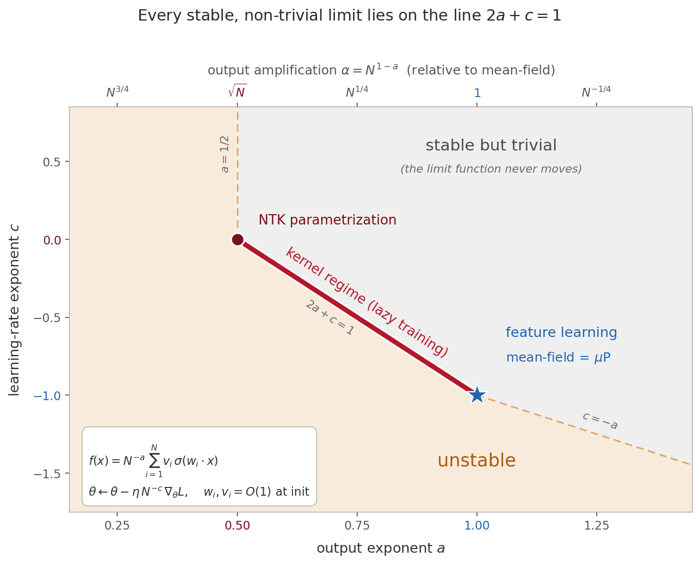
Yang and Hu’s dynamical dichotomy theorem says that every abc-parametrization admitting a stable, nontrivial infinite-width limit lands in one of exactly two phases: the lazy phase or the feature-learning phase. There are no alternatives. The mean-field and NTK parameterizations are revealed to be just two choices among the broader landscape of possible parameterizations.

It helps to think about how the exponents encourage feature learning. Let’s assume that we keep $b$ fixed at zero, so that our parameters are $O(1)$ at initialization. In general, if you want feature learning, you want a larger $a$ and smaller $c$. Larger $a$ means the output is scaled down, so the function has to travel further in function space to fit the target. And smaller $c$ means the learning rate is larger, so each iteration of gradient descent causes a larger change in the parameters.

Within the feature-learning phase there is a distinguished point, the maximal update parametrization ($\mu$P), at which every layer’s features move at the largest stable rate. $\mu$P has since become a practical tool. Using $\mu$P, you can tune hyperparameters on smaller models and then transfer them to a large one.

Below is a phase diagram for the abc-parametrization of the two-layer neural network. Because the abc-parametrization has a built-in redundancy, we can depict the relevant phases while varying only two of the scaling exponents. We will work with the coordinates $(a,c)$. If you fix the initialization at its standard $O(1)$ scale, then the parametrizations corresponding to nontrivial infinite-width limits all lie on the line $2a + c = 1$. The NTK parametrization sits at $(1/2, 0)$ and the mean-field parametrization at $(1,-1)$.

Beyond Two Layers

While mean-field theory for two-layer neural networks is well understood, extending it beyond two layers has proved more delicate. In a two-layer network the neurons enter exchangeably, so the state of the system is captured by a single measure on $\mathbb{R}^{d+1}$. Unfortunately, that is no longer true for deeper networks.

Rigorous multi-layer mean-field limits do exist. Sirignano and Spiliopoulos (2019), Araújo, Oliveira, and Yukimura (2019), and Nguyen and Pham (2020) all constructed versions. But the mathematical objects are heavier.

In practice, the scaling perspective has proved quite useful. Yang’s Tensor Programs framework handles arbitrary architectures by asking about scaling exponents rather than particle densities. Its physics falls out of a practitioner’s question: how large a learning rate should each layer get? Demand feature learning everywhere and one obtains the maximal update parametrization—which for two-layer networks returns the mean-field parametrization exactly.