'A High-Bias, Low-Variance Introduction to Machine Learning for Physicists' by Pankaj Mehta

Pankaj Mehta is a theoretical physicist at Boston University who specializes in biophysics and statistical physics. In 2019, together with his six co-authors, he published a set of lecture notes: A high-bias, low-variance introduction to Machine Learning for physicists.

Last year, I reviewed Jared Kaplan’s machine learning lecture notes. It’s interesting to compare and contrast the two sets of notes. Both are introductions to machine learning written by a physicist for other physicists. But Kaplan’s notes, as well-written as they are, ultimately read like a by-the-numbers introductory machine learning textbook. Mehta’s notes, on the other hand, are more experimental in that they really try to take their target audience seriously. They attempt something bold: to recast machine learning as a subfield of statistical physics.

(Throughout, whenever I say “Mehta” I really mean “Mehta et al” but I’ll abbreviate for readability.)

The notes open with a rallying cry for why physicists are natural contributors to machine learning:

Physicists are uniquely situated to benefit from and contribute to ML. Many of the core concepts and techniques used in ML—such as Monte-Carlo methods, simulated annealing, variational methods—have their origins in physics. Moreover, “energy-based models” inspired by statistical physics are the backbone of many deep learning methods. For these reasons, there is much in modern ML that will be familiar to physicists. Physicists and astronomers have also been at the forefront of using “big data”. For example, experiments such as CMS and ATLAS at the LHC generate petabytes of data per year. In astronomy, projects such as the Sloan Digital Sky Survey (SDSS) routinely analyze and release hundreds of terabytes of data measuring the properties of nearly a billion stars and galaxies. Researchers in these fields are increasingly incorporating recent advances in ML and data science, and this trend is likely to accelerate in the future.

It’s a thread emphasized throughout: whenever he has a chance, Mehta draws a connection between the machine learning concept he is introducing and a related idea from physics.

One caveat on scope: the book only covers supervised and unsupervised learning. The authors chose to forgo reinforcement learning in order to make the lecture notes more cohesive.

The Bias-Variance Tradeoff

The book starts by reviewing the basics of statistical learning theory: machine learning as high-dimensional parametrized statistics.

The core difficulty is generalization: we train models to minimize error on the training set, but what we actually want is high performance on data the model has never seen.

Consider the setting of supervised learning. We are given a data distribution $\mu$ over $\mathbb{R}^d \times \mathbb{R}$, from which we draw input-output pairs $(x, y) \sim \mu$. Our goal is to learn the target function $f$, defined as the conditional expectation of the output given the input:

\[f(x) = \mathbb{E}[y \mid x]\]

It’s the function $f$ that we would like our supervised model $\hat{f}(x; \theta)$ to learn. Even when the outputs are noisy, the conditional expectation is a deterministic function of the input. For simplicity, we will assume homoscedastic noise: $y = f(x) + \epsilon$, where $\epsilon$ has mean zero and variance $\sigma^2$ at every $x$.

We train on a data set $\mathcal{D}$ consisting of $N$ independent and identically distributed draws from the larger distribution $\mu$. What’s important is that $\mathcal{D}$ is random: some draws are more representative than others.

Let $E_{in}$ be the model’s error on the training set and $E_{out}$ be its expected error on fresh data. We use $\mathcal{D}$ to minimize the training error $E_{in}$, and by doing so we obtain the final learned parameters $\hat{\theta}_{\mathcal{D}}$. Because $\mathcal{D}$ is random, $\hat{\theta}_{\mathcal{D}}$ is random as well.

And importantly, because the final learned parameters are random, the generalization error is random too. Sometimes you receive a favorable data set and generalize well. Sometimes you receive an unrepresentative one and generalize poorly. The interesting object is therefore $E_{out}$ averaged over everything random: the draw of the training set and the noise on the outputs.

\[\begin{align} \mathbb{E}_{\mathcal{D}}[E_{out}] &= \mathbb{E}_{\mathcal{D}, x, \epsilon} \left[ \left( y - \hat{f}_{\mathcal{D}}(x) \right)^2 \right] \\ &= \mathbb{E}_{\mathcal{D}, x, \epsilon} \left[ \left( \epsilon + f(x) - \hat{f}_{\mathcal{D}}(x) \right)^2 \right] \end{align}\]

where $\hat{f}_{\mathcal{D}}(x) \equiv \hat{f}(x; \hat{\theta}_{\mathcal{D}})$ is the model we end up with after training on the draw $\mathcal{D}$.

For any random variable $Z$ we can decompose the second moment into the square of the first moment plus the variance:

\[\langle Z^2 \rangle = \langle Z \rangle^2 + \left\langle \left( Z - \langle Z \rangle \right)^2 \right\rangle\]

Here $Z$ is the residual $f(x) - \hat{f}_{\mathcal{D}}(x)$ at a fixed test point $x$, viewed as a random variable over draws of $\mathcal{D}$. When you expand the square in our expression for the generalization error, the cross terms in $\epsilon$ drop out because the noise has mean zero at every $x$ and is independent of the training set. What survives is a sum of three non-negative pieces:

\[\mathbb{E}_{\mathcal{D}}[E_{out}] = \sigma^2 + \mathbb{E}_x \left[ \left( f(x) - \mathbb{E}_{\mathcal{D}} \left[ \hat{f}_{\mathcal{D}}(x) \right] \right)^2 \right] + \mathbb{E}_x \left[ \mathbb{E}_{\mathcal{D}} \left[ \left( \hat{f}_{\mathcal{D}}(x) - \mathbb{E}_{\mathcal{D}} \left[ \hat{f}_{\mathcal{D}}(x) \right] \right)^2 \right] \right]\]

The first term is irreducible noise: no choice of model makes it go away. The second is the bias squared: how far the average fitted model sits from the target function. The third is the variance: how much the fitted model varies from one realization of the data set to the next. This is the bias-variance decomposition of the generalization error.

It’s a tradeoff because the two error sources respond oppositely to a key choice: how expressive to make the model class.

The expressiveness of a model class is roughly how many different functions it can represent. A class with low expressiveness can represent only a limited number of functions. Because it often can’t represent the target function at all, the bias is large. But precisely because it has few degrees of freedom, it barely notices which draw of $\mathcal{D}$ it was handed, so the variance of the fitted function is small.

A highly expressive class, by contrast, can represent many different functions. This makes it more likely that one of them is close to the target—so the bias is small. But the fit also begins to chase the noise in whichever data set it happened to see—so the variance is large. Because $E_{out}$ is the sum of the squared bias and the variance (plus the irreducible $\sigma^2$), it is typically U-shaped in model complexity: the optimal complexity is not the one that fits the training data best, but the one that balances bias against variance.

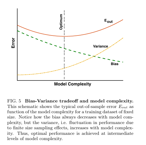
Figure from Mehta 2019

Regularization is another way to navigate the bias-variance tradeoff. With regularization, instead of minimizing the loss $L(\theta)$, you minimize the loss plus a penalty on the size of the parameters. The two standard choices are the $\ell_2$ penalty of ridge regression and the $\ell_1$ penalty of lasso regression:

\[L_{\text{ridge}}(\theta) = L(\theta) + \lambda \|\theta\|_2^2, \qquad L_{\text{lasso}}(\theta) = L(\theta) + \lambda \|\theta\|_1\]

A helpful way to see what the penalties do—which is exact for a convex loss—is through the lens of constrained optimization: minimizing the penalized loss amounts to minimizing the unregularized loss subject to the parameters lying in a region around the origin—a round disk for ridge regression and a diamond for lasso regression.

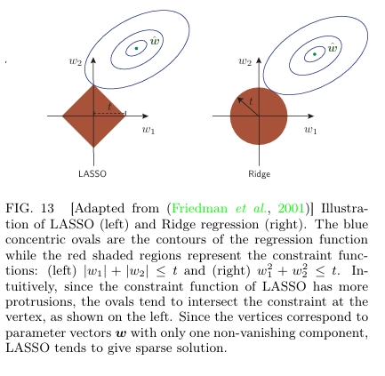
Figure from Mehta 2019, adapted from Friedman et al. 2001

In bias-variance terms, the strength of the regularization dictates where you sit on the tradeoff. Increasing the regularization shrinks the solution set, so different realizations of the data obtain more similar models. This causes the variance goes down. But if the regularization is too strong, the target function will have features that no small-norm parameter vector can express. You will never learn those features no matter how much data you train on—which causes the asymptotic bias to go up. The sweet spot will be somewhere in between no regularization and infinite regularization.

Let’s look at a concrete example. Consider a target function $x^2 + x$, which we try to fit with a degree-ten polynomial. Because we are heavily overparameterized, with no regularization we overfit quite badly—a manifestation of the variance term in the generalization error. But we can now introduce a regularization parameter.

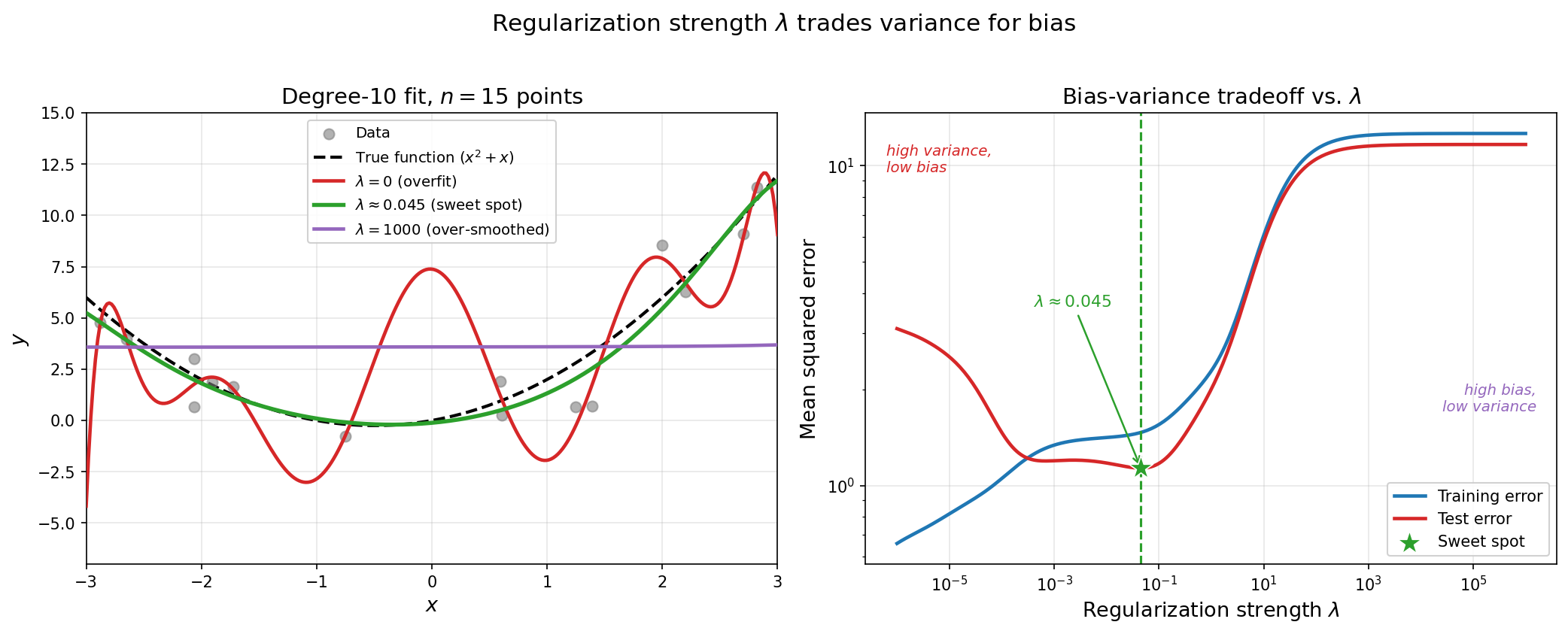
At $\lambda = 0$, the fitted function oscillates wildly, overfitting to the noise. At $\lambda = 1000$, the fitted function flattens into a constant function equal to the mean of the training set. With a carefully chosen $\lambda$, we can minimize the test error and recover the target function.

The Ising Model Organism

The book doesn’t just want you to read about the concepts, but to also see them in action with real data. So at the end of each chapter, whatever concept was just introduced gets exercised on key examples. Accompanying the book is a set of Jupyter notebooks.

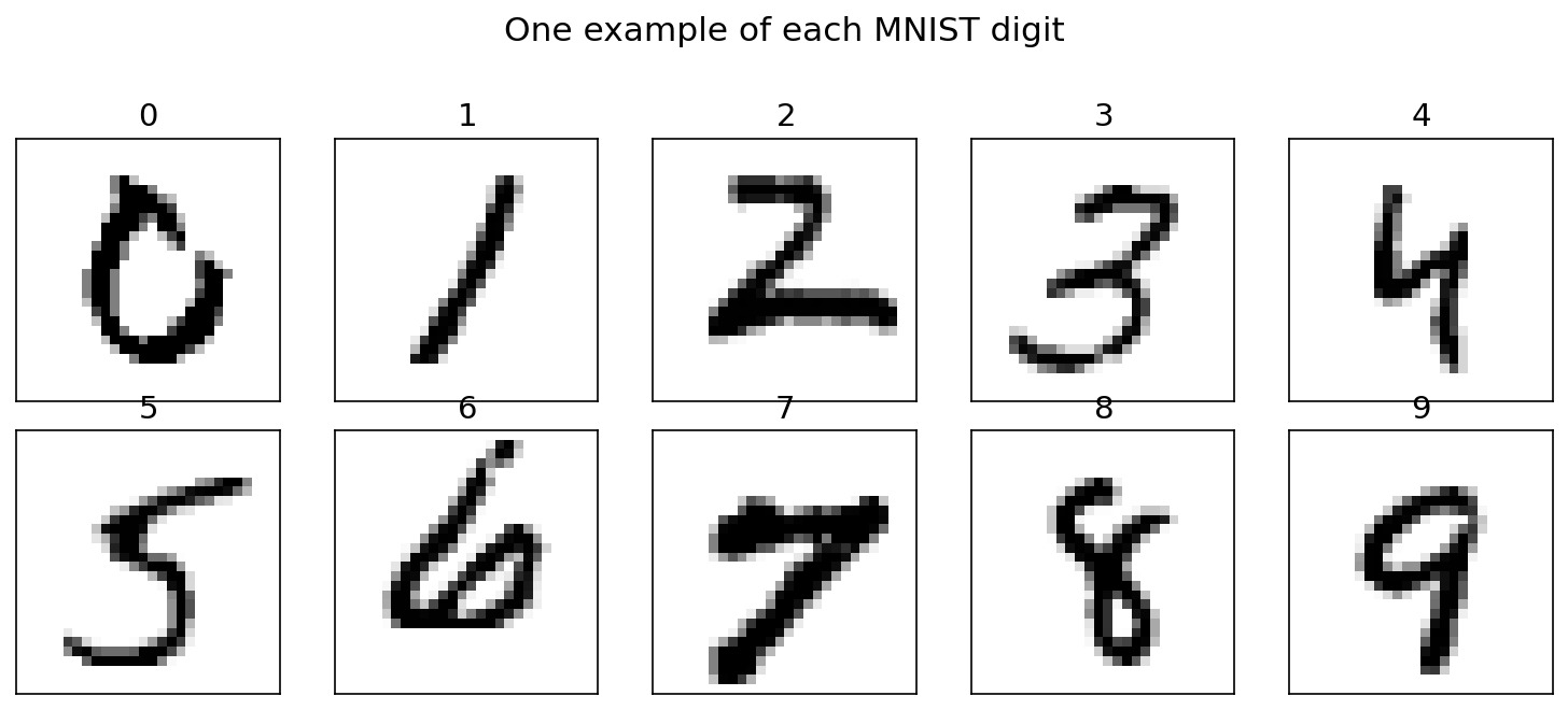
Three data sets run through the book. The first is MNIST, a collection of handwritten digits. You can use it for unsupervised tasks like clustering or for supervised ones like classification.

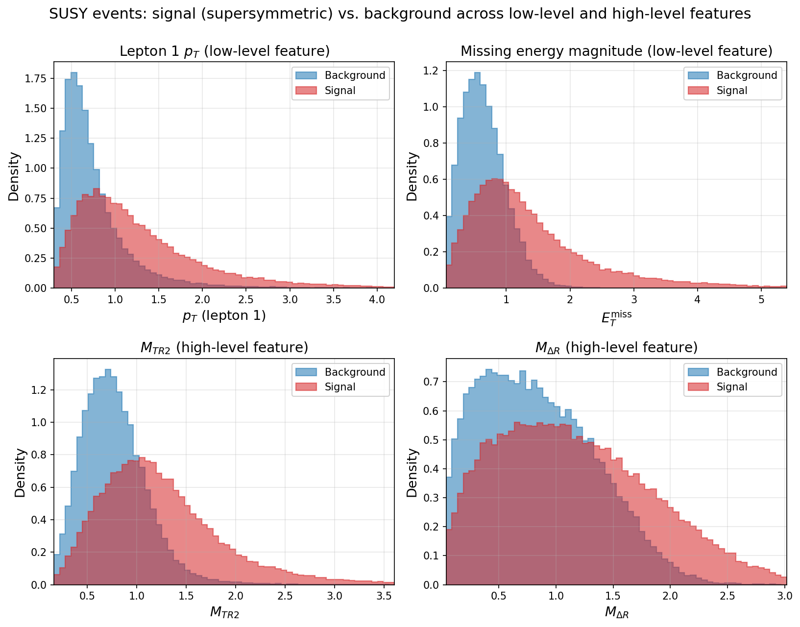
Another data set is SUSY, from Baldi, Sadowski, and Whiteson’s 2014 paper on deep learning in high-energy physics. It consists of five million proton-proton collision events—simulated rather than real—and the task is to classify whether a collision produced supersymmetric particles.

What makes the task subtle is that the observable end products—the protons—are the same whether or not the collision produced supersymmetric particles. Only the kinematics—the outgoing momenta, for instance—differ between the two classes. Each event carries 18 features: 8 low-level kinematic ones, plus 10 high-level features hand-engineered by physicists using their knowledge of what signatures a supersymmetric decay should leave. The punchline is that neural networks reach comparable performance when trained using only the low-level features—whatever the hand-crafted features were adding, the network rediscovers it over the course of training.

But the most iconic data set in the book is easily the Ising model. The Ising model is the model organism of statistical physics: whenever a statistical physicist wants to understand a new concept, they reach for their trusty Ising model. The book imports that ritual wholesale.

The Ising model was introduced as a minimal model of magnetism. The system lives on a lattice, with a little spin at every site that can point either up or down. A helpful cartoon is to imagine a particle spinning about its axis—counterclockwise with its magnetic moment pointing up, or clockwise with it pointing down:

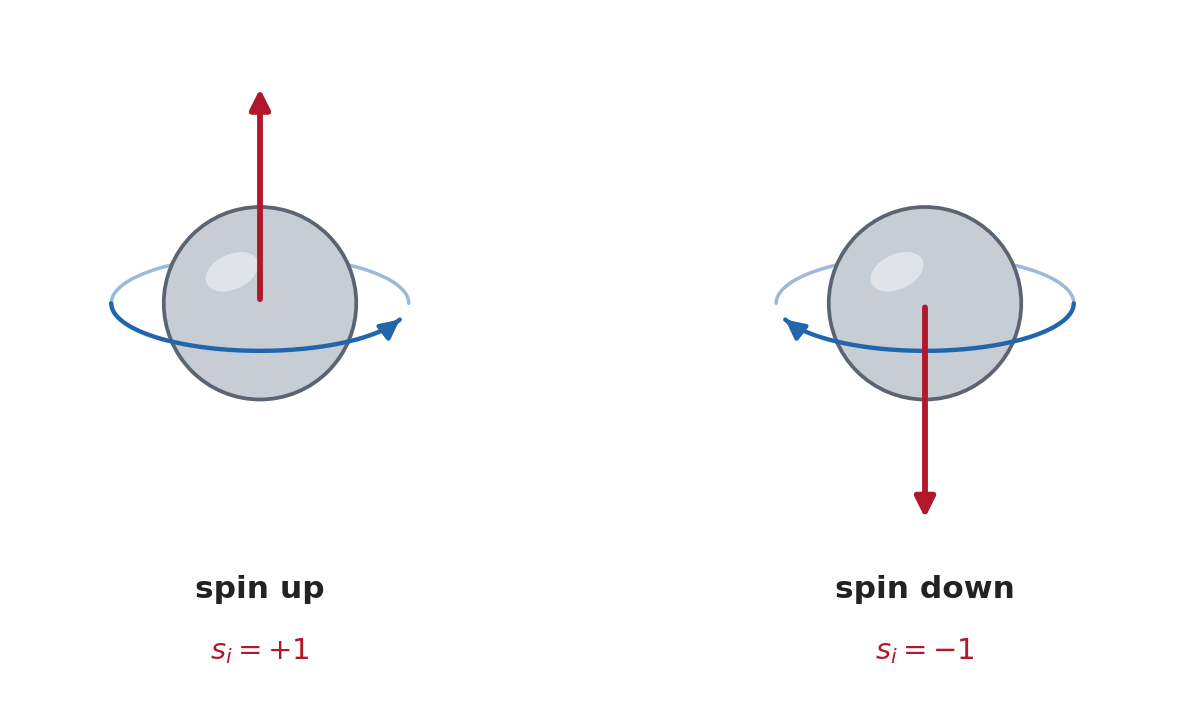
The key question is this: if each lattice site has a little magnetic moment, how do those add up to the macroscopic magnetism we observe? If every spin pointed in a random direction, the average magnetization would be zero and there would be no macroscopic magnetization at all.

The assumption the Ising model makes is that neighboring spins want to align with each other: if one spin points up, that encourages its neighbors to point up too (and likewise for down). The way to encode this preference is through the energy function—the Hamiltonian:

\[E = -J \sum_{\langle i j \rangle} s_i s_j\]

where the spins take values $s_i = \pm 1$. The sum runs over nearest-neighbor pairs $\langle i j \rangle$, and $J > 0$ is the coupling constant. Physical systems like to sit in low-energy states, so the minus sign means that the energy drops when neighboring spins are pointed in the same direction: alignment is rewarded.

How do we use the Ising model to generate data? By sampling from its Boltzmann distribution. Even though systems prefer low-energy configurations, at any finite temperature there is some probability of finding the system in a higher-energy one. The higher the temperature, the more likely those configurations become. This is encapsulated in the Boltzmann distribution:

\[p(\lbrace s_i \rbrace) \propto e^{-E/T}\]

To generate data, we sample from this distribution—drawing random Ising model configurations. Most of the book’s Ising examples use the 2D model on a $40 \times 40$ lattice. Because the Boltzmann distribution depends only on the ratio $J/T$, the book sets $J = 1$ and varies $T$ as needed.

What learning tasks can you do once you have Ising-model-generated data? One example is linear regression. Suppose I hand you spin configurations $\lbrace s_i \rbrace$ together with their energies $E[\lbrace s_i \rbrace]$, and ask you to infer the Hamiltonian that generated them. Our model class is given as:

\[E_{\widehat{J}}[\{s_i\}] = -\sum_{i, j} \widehat{J}_{ij} \, s_i s_j.\]

The class of Hamiltonians is constrained to quadratic forms. However, the space of allowable coupling matrices $\widehat{J}$ includes any square matrix. Let $\mathcal{D} = \lbrace (\lbrace s_i \rbrace^{(n)}, E^{(n)}) \rbrace_{n=1}^N$ be our data set of configurations and their energies. The loss is then

\[L(\widehat{J}) = \sum_{n=1}^{N} \Big( E^{(n)} - H_{\widehat{J}}[\{s_i\}^{(n)}] \Big)^2.\]

This is precisely linear regression: the pairwise products $s_i s_j$ are the features and the couplings $\widehat{J}_{ij}$ are the regression coefficients.

While ordinary least squares does a passable job of predicting energies, it is suboptimal. The true couplings are symmetric, $J_{ij} = J_{ji}$, but nothing constrains the fitted $\widehat{J}$ to be symmetric. Worse, the data can’t enforce symmetry either: since $s_i s_j = s_j s_i$, the energy depends only on the sum $\widehat{J}_{ij} + \widehat{J}_{ji}$. The antisymmetric part of $\widehat{J}$ is invisible to the loss.

And the true coupling matrix has still yet more structure that a raw fit has no way to exploit: it is sparse—only the nearest-neighbor entries are nonzero. But thankfully, this is exactly the setting where regularization can help.

Recall that lasso regression can be viewed as constrained optimization, with the set of allowed solutions confined to a diamond. It turns out that this shape is very special. Imagine that the point minimizing the training error lies outside the diamond. Surrounding that point are level sets of increasing loss, radiating outwards. Because of the diamond’s shape, the first level set to touch the allowed region will tend to touch it at a corner—and the corners are exactly the points where some subset of the parameters are not merely small but strictly zero. So lasso doesn’t just shrink the fitted parameters—it induces a preference for setting them to exactly zero.

Another task we can use the Ising-model-generated data for is classifying phases. Magnets have two phases: a high-temperature phase in which the spins are not aligned and there is no net magnetization, and a low-temperature phase in which they are aligned and there is a net magnetization. The transition between the two regimes happens sharply at a critical temperature $T_c$. As a classification task, we can set up the Ising model at a high temperature and at a low temperature and sample configurations from each. We then train a model to distinguish between configurations drawn from the two phases.

There is an interesting and well-known history among physicists regarding the Ising model and phase transitions. Wilhelm Lenz first proposed the model in 1920 as a minimal model of a magnet. He then handed it to his doctoral student, Ernst Ising, who solved the one-dimensional version in 1924 for his PhD dissertation. Ising found, to everyone’s disappointment, no phase transition: the 1D model never magnetizes at finite temperature. The magnetized phase everyone was looking for finally appeared in 1944, when Lars Onsager solved the two-dimensional model exactly and found a genuine phase transition.

To this day, the three-dimensional Ising model has resisted exact solution, despite plenty of attempts. That is not to say we know nothing about it: the phase transition is rigorously established, and its critical exponents—the powers governing how thermodynamic quantities diverge or vanish at the phase transition—are known to many decimal places thanks to Monte Carlo and the conformal bootstrap. What’s missing is a closed-form solution. Above four dimensions, by contrast, the problem becomes easy again: fluctuations stop mattering near the critical point, and the critical exponents collapse to their mean-field values.

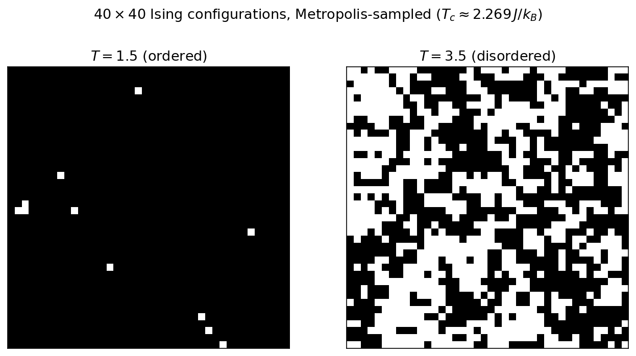
A human can assign these two configurations to their correct phase at a glance. But how do you get a machine to do it?

We could attempt our usual mean-squared-error approach for supervised learning. The data take the form $(\lbrace s_i \rbrace, y)$, where $\lbrace s_i \rbrace$ is the configuration and $y$ is a label denoting the phase: $y = 1$ in the high-temperature phase and $y = 0$ in the low-temperature phase. We then set up linear regression with the fitted function interpreted as the probability that the configuration came from the high-temperature phase.

However, there are problems with this approach. For one, we want the output to be interpreted as a probability, but a linear model’s range spans the entire real line, allowing negative probabilities and probabilities greater than one. Another issue is that a linear model treats all regions of the range alike. Ideally the model’s probability should move readily near 50% and become harder and harder to shift as it approaches 0% or 100%. With linear regression, going from 50% to 51% is exactly as easy as going from 98% to 99%.

An alternative is logistic regression: a linear model whose output is not the probability itself but the log-odds, or logit, of being in the high-temperature phase. For a probability $p$, the logit is

\[z = \operatorname{logit}(p) = \log \left (\frac{p}{1 - p} \right ).\]

As $p$ ranges over $(0, 1)$, $z$ ranges over the whole real line: $z \to -\infty$ as $p \to 0$, $z \to +\infty$ as $p \to 1$, and $z = 0$ at $p = 1/2$. Because it’s uncontrained, it’s sensible for the linear model to predict $z$. We can then recover the probability by inverting:

\[p = \sigma(z) = \frac{1}{1 + e^{-z}},\]

where $\sigma$ is the logistic function.

However, there’s now a new issue. Our labels are exactly $0$ and $1$, and the logit of $0$ or $1$ is $\mp\infty$. So we can’t simply transform the targets into log-odds and run least squares on them.

The fix is to transform the model rather than the data. Whereas before our model encoded a function—the conditional expectation of $y$ given $x$—it will now encode a conditional distribution $p(y \mid x)$. And once a model specifies a distribution, there is a canonical objective: maximum likelihood. Writing $x$ for the configuration $\lbrace s_i \rbrace$, the negative log-likelihood of a data set $\mathcal{D} = \lbrace (x^{(n)}, y^{(n)}) \rbrace$ is

\[L(\theta) = -\sum_{n} \Big[ y^{(n)} \log \sigma(z^{(n)}) + (1 - y^{(n)}) \log\big(1 - \sigma(z^{(n)})\big) \Big].\]

This is the cross-entropy loss. Each term in the sum is the cross-entropy between the observed label—a point mass at $y^{(n)}$—and the model’s predicted distribution. Averaged over the data, minimizing it is the same as minimizing the KL divergence of the data’s conditional distribution $p(y \mid x)$ from the model’s $p_\theta(y \mid x)$:

\[\begin{align} KL(p \| p_\theta) &= \sum_y p(y \mid x) \log \frac{p(y \mid x)}{p_\theta(y \mid x)} \\ &= \sum_y p(y \mid x) \log p(y \mid x) - \sum_y p(y \mid x) \log p_\theta(y \mid x) \\ &= -H(p) + H(p, p_\theta), \end{align}\]

where

\[H(p) = -\sum_y p(y \mid x) \log p(y \mid x)\]

is the entropy of the data and

\[H(p, p_\theta) = -\sum_y p(y \mid x) \log p_\theta(y \mid x)\]

is the cross-entropy. (An unfortunate collision with the Hamiltonian’s $H$, but both usages are standard.)

The data’s entropy is independent of $\theta$, so the model-dependent part of the KL divergence is precisely the cross-entropy. Minimize one and you minimize the other. And unlike the squared error between two probabilities, which can never exceed 1, the cross-entropy diverges when the model is confidently wrong.

Machine Learning From a Physics Point-of-View

Mehta observes that a hallmark of physics is the exploitation of known structure—symmetries, locality—to make progress.

One of the core lessons of physics is that we should exploit symmetries and invariances when analyzing physical systems. Properties such as locality and translational invariance are often built directly into the physical laws. […] This basic idea, tailoring our analysis to exploit additional structure, is a key feature of modern physical theories from general relativity, through gauge theories, to critical phenomena.

He argues that the same principle explains what alternative neural network architectures give you over the standard MLP: data sets have structure too, and an architecture is a way of building that structure in.

Like physical systems, many datasets and supervised learning tasks also possess additional symmetries and structure. […] Because a cat is a physical object, we know that these features are likely to be local (groups of neighboring pixels in the two-dimensional image corresponding to whiskers, tails, eyes, etc). We also know that the cat can be anywhere in the image. […] This example makes clear that, like many physical systems, many ML tasks (especially in the context of computer vision and image processing) also possess additional structure, such as locality and translation invariance.

We can contextualize this with respect to the bias-variance tradeoff. The tradeoff says that generalization error decomposes into bias and variance, and that raising or lowering the model complexity moves you along the curve. The intuition for why lower complexity means higher bias is that a smaller hypothesis space is more likely to exclude the true hypothesis altogether.

But that intuition assumes you shrink the hypothesis space blindly. If you know something about the problem—that the features are local or that the answer shouldn’t change when the image is shifted—you can discard hypotheses that were never going to be right anyway. You would then get the variance reduction of a smaller model class without paying the usual price in bias. This is the inductive bias of the model class: the hypotheses it prefers before it has seen any data.

Consider the convolutional neural network (CNN). Suppose the input is an image and the task is to classify it. The image comes naturally arranged on a two-dimensional grid—and CNNs are built to exploit that.

There are two types of layer in a CNN. There are convolutional layers which slide a small learned filter across the previous layer, computing the same weighted sum at every position. There are also pooling layers which shrink the spatial dimensions, aggregating each neighborhood into a single value. (Somewhat humorously, the book’s own figure relabels the pooling step using language more familiar to a physicist: coarse-graining.)

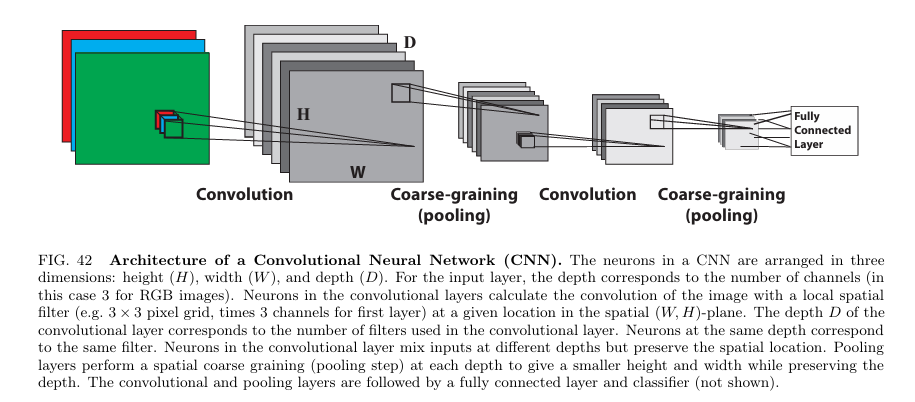
Figure from Mehta 2019

A convolution is a mathematical operation that takes two functions and combines them, creating a third function. Given functions $f$ and $g$, it is defined as

\[(f \ast g)(y) = \int dx \, f(x) \, g(y - x)\]

For each output point $y$, you slide the filter $g$ over $f$, weight the values of $f$ by it, and sum.

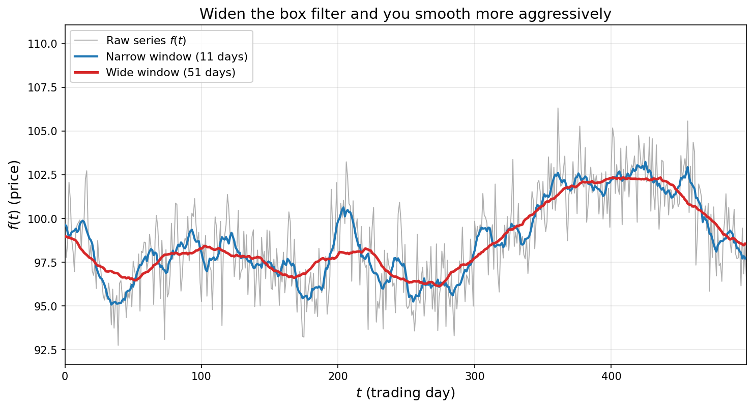
A familiar example is the moving average. In a noisy time series—like stock prices—we often care more about the average trend than we do about the value at any one instant. Taking $f(t)$ to be the time series and letting

\[g(t) = \frac{1}{2c} \, \Theta(c - |t|)\]

to be the filter, the convolution $(f \ast g)(t)$ returns the average of $f$ over the window $[t - c, \, t + c]$. Widen the box and you smooth more aggressively. Narrow it and you keep more of the fluctuation. In a CNN, the filter $g$ is learnable, parameterized by the weights of the network.

A generic feed-forward network connects everything in the previous layer to everything else. By contrast a CNN, by being built on convolution, bakes two assumptions directly into its architecture. It encodes locality because each neuron only sees a small spatial patch of the previous layer. And it encodes translation invariance because the same filter weights are shared across the entire layer.

The Ising model is a perfect test case for the CNN because its physics also exhibits both locality and translation-invariance: the Hamiltonian couples only the nearest neighbors, and it looks the same at every lattice site. And indeed: when applied to the phase classification task, the CNN outperforms the MLP—while using fewer parameters to boot.

Now consider energy-based models. These are generative models: models that learn a probability distribution so that you can sample from the distribution during inference.

An energy-based model isn’t an architecture like a CNN. Energy-based models can be built on a wide variety of architectures, including MLPs, CNNs, or transformers. What the term specifies is a choice about what the network represents. Here, the network encodes an energy function: a map from configurations to scalars.

\[E_\theta: \mathcal{X} \rightarrow \mathbb{R}\]

And the distribution the model represents is the Boltzmann distribution of that energy:

\[p_\theta(x) = \frac{e^{-E_\theta(x)}}{Z_\theta}, \qquad Z_\theta = \sum_x e^{-E_\theta(x)}\]

where the partition function $Z_\theta$ acts as a normalizing constant. (Note that Boltzmann distributions usually involve a temperature, but we’ve implicitly absorbed the temperature into the definition of the energy itself.) With Boltzmann distributions, lower energy corresponds to higher probability, and higher energy corresponds to lower probability.

But why should the distribution take the form of a Boltzmann distribution? One justification is the maximum entropy principle: the idea that the distribution we should choose is the one that maximizes entropy subject to the constraint of fixing the expected energy.

Consider the following functional over the space of measures on our input space:

\[\mathcal{S}[\mu] = S[\mu] - \frac{1}{T}\big(\langle E \rangle_\mu - E_0\big)\]

We would like to maximize this functional. The first term is the entropy. The second term encodes our constraint: here $1/T$ acts as a Lagrange multiplier, enforcing that our distribution $\mu$ has the correct expected energy $E_0$. The maximizing distribution of this functional is precisely the Boltzmann distribution.

How do you train an energy-based model? The model specifies a distribution, so the canonical loss function is once again the cross entropy.

\[\begin{align} L(\theta) &= -\langle \log p_\theta(x) \rangle_{\text{data}} \\ &= \langle E_\theta(x) \rangle_{\text{data}} + \log Z_\theta \end{align}\]

where $\langle \cdot \rangle_{\text{data}}$ denotes an average over the training set. The first term is easy to evaluate. But the second term is problematic. Computing the partition function requires summing over every configuration—intractable for anything but toy models.

But if you differentiate $\log Z_\theta$ with respect to $\theta$, you can obtain a more tractable expression.

\[\begin{align} \nabla_\theta \log Z_\theta &= \frac{1}{Z_\theta}\nabla_\theta Z_\theta \\ &= \frac{1}{Z_\theta}\nabla_\theta \int e^{-E_\theta(x)}\,dx \\ &= \int \frac{e^{-E_\theta(x)}}{Z_\theta}\big(-\nabla_\theta E_\theta(x)\big)\,dx \\ &= -\big\langle \nabla_\theta E_\theta(x) \big\rangle_{p_\theta} \\ \end{align}\]

While the new expression no longer explicitly involves the partition function, it is still difficult to compute: estimating it requires sampling from the model distribution via MCMC. Substituting the found expression into the loss, the gradient becomes a difference of two expectations:

\[\nabla_\theta L = \langle \nabla_\theta E_\theta(x) \rangle_{\text{data}} - \langle \nabla_\theta E_\theta(x) \rangle_{p_\theta}\]

The first expectation—which is with respect to the data—is called the positive phase. The second expectation—which is with respect to the model distribution—is called the negative phase. The loss function is contrastive: the model must update such that the energy of real data is pushed down, and the energy of the model’s own samples are pushed up.

Now let’s consider the special case where the energy is linear in the parameters: a linear combination of pre-selected features, with the coefficients being learnable.

\[E_\theta(x) = \sum_m \theta_m f_m(x)\]

We then have for the gradient of our loss function:

\[\frac{\partial \mathcal{L}}{\partial \theta_m} = \langle f_m \rangle_{\text{model}} - \langle f_m \rangle_{\text{data}}\]

So at any critical point the model reproduces the empirical expectation of every feature:

\[\langle f_m \rangle_{\text{model}} = \langle f_m \rangle_{\text{data}}\]

These are moment-matching conditions. The maximum-entropy distribution consistent with them is exactly the Boltzmann distribution whose energy is a linear combination of the features—with the parameters playing the role of the Lagrange multipliers.

But which features should you constrain? Naively, the more aspects of the data you pin down, the better the fit. But recall the bias-variance tradeoff. With a finite sample, the empirical expectation of each feature is noisy. Constrain a feature whose empirical average is unreliable and you end up fitting noise. But on the other hand, if leave out a feature that matters, no amount of data will recover the right distribution. Choosing which moments of the data to trust is an example of feature engineering—and it’s a generically hard problem.

One principled choice is to preferentially constrain lower-order terms. Consider a system of $N$ binary variables $\lbrace s_i \rbrace$. Suppose we constrain only the means $\langle s_i \rangle$ and the pairwise correlations $\langle s_i s_j \rangle$ to match their observed values. The maximum-entropy distribution consistent with those constraints has an energy of the form:

\[E(\lbrace s_i \rbrace) = -\sum_i h_i s_i - \sum_{i<j} J_{ij} s_i s_j\]

This is precisely a generalized Ising model! This is only one example of the multitude of connections between statistical mechanics and graphical models.

One of the deeper chapters of the book is on variational methods. If you think about it, everything hard about energy-based models traces back to the intractability of the partition function. During training, it forces us to use MCMC for the negative phase. At inference, MCMC is the only way to sample from the model at all. And this is a generic problem—for an arbitrary energy function, the associated partition function will be intractable.

One workaround is to give up on the true distribution and learn instead the closest member of some family of distributions whose partition functions you can compute. This is called a variational approximation.

A classic example from physics is mean-field theory: you replace the intractable distribution with the closest-matching product measure—one in which all the random variables are independent. “Closest-matching” here means the product measure $q$ minimizing the KL divergence $KL(q \Vert p)$ from the true distribution $p$.

For the Ising model, this variational principle gives rise to a set of self-consistent mean-field equations. Consider a generalized Ising model, with energy function:

\[E(s) = -\sum_{i<j} J_{ij} s_i s_j - \sum_i h_i s_i\]

For a single binary variable, the distribution is uniquely determined by its mean—with the mean corresponding to how “biased” the coin flip is. For a single spin $s_i$ with expectation $m_i = \langle s_i \rangle$, we have for its distribution:

\[q_i(s_i) = \frac{1 + m_is_i}{2}\]

A product measure over all the spins is then just the product of these single-spin distributions:

\[q(s) = \prod_i \frac{1 + m_i s_i}{2}\]

The family of product measures is parameterized by the $N$-dimensional vector of means $m$. Evaluating $KL(q \Vert p)$, we have that:

\[\begin{align} KL(q \Vert p) &= \sum_s q(s) \log \frac{q(s)}{p(s)} \\[4pt] &= \sum_s q(s) \log q(s) - \sum_s q(s) \log p(s) \\[4pt] &= -H(q) + \sum_s q(s)\big(\beta E(s) + \log Z\big) \\[4pt] &= \beta \langle E \rangle_q - H(q) + \log Z \\[4pt] &= \beta\Big(\langle E \rangle_q - \tfrac{1}{\beta} H(q)\Big) + \log Z \end{align}\]

So minimizing $KL(q \Vert p)$ over this family is the same as minimizing the variational free energy:

\[F[q] = \langle E \rangle_q - \frac{1}{\beta}H(q)\]

The two differ only by a factor of $\beta$ and a $\log Z$ term—neither of which depends on $q$.

Both terms in the variational free energy are tractable. Setting $\partial F / \partial m_i = 0$, yields a set of self-consistent mean-field equations for the magnetizations.

\[m_i = \tanh\Big(\beta \Big(h_i + \sum_{j \neq i} J_{ij} m_j\Big)\Big)\]

It’s called mean-field because each spin feels its neighbors only through their average values over the ensemble, independent of the specific realization of the configuration.

Miscellaneous

The book covers a lot of other material. It spends a chapter on ensemble methods—combining many models into one. The motivation behind ensembling is once again the bias-variance tradeoff: averaging over many models cancels the part of the error that varies from one training set to the next.

It also covers various unsupervised methods for dimensionality reduction and visualization, such as principal component analysis, multidimensional scaling, and t-SNE. A further chapter takes up clustering—how to sort data points into groups. The canonical algorithm is k-means: alternately assign each point to its nearest cluster center, then move each center to the mean of the points assigned to it.

In any case, the book successfully articulates many of the close connections between machine learning and statistical physics.