Pre-Conditioners Are Just Metric Tensors

While gradient descent is the simplest optimization algorithm, it’s rarely the optimization algorithm that is actually used in practice. In machine learning, a common way in which optimizers are modified is the use of a preconditioner: rather than updating the parameters with the raw gradient, a preconditioner $P$ applies a matrix to the gradient before adding it to the parameters.

\[\theta_{t+1} = \theta_t - \eta P^{-1} \nabla_\theta L\]

That we apply $P^{-1}$, not $P$, to the gradient of the loss is conventional—a convention that I will soon argue is conceptually well-motivated.

Why would we want preconditioners? One reason is that rather than having one global step size, we want to be able to take different-sized steps in different directions based on the curvature of the loss. This gets around a core problem of using a single global learning rate: if the learning rate is too large relative to the curvature in a given direction, the optimizer will oscillate rather than converge. So a single global learning rate must be small enough for the sharpest direction of the Hessian, which means it will be unnecessarily small for the flatter directions. With a preconditioner, you can take smaller steps in sharper directions and larger steps in flatter directions.

Vanilla gradient descent is a first-order method: it only uses the gradient (the first derivative of the loss). Methods that use curvature information—that is, information about the second derivatives of the loss—are called second-order methods. Many of the preconditioners actually used in machine learning can be understood as cheap approximations to second-order methods—they try to capture the benefits of curvature information without the full cost of computing the Hessian.

While the case for preconditioners is quite practical, they also have a very clean geometric interpretation: the matrix $P$ plays the role of the metric tensor on parameter space.

The Metric Tensor

Vanilla gradient descent is actually a bit strange from a mathematical perspective: it adds two things of unlike types.

Consider the standard gradient descent update rule, rearranged slightly:

\[\theta_{t+1} - \theta_t = - \eta \nabla L\]

The left-hand side is a displacement between consecutive parameter values—it is a vector. A vector represents a direction and magnitude in parameter space. The right-hand side is the gradient of the loss function—which is a covector. A covector is a quantity that takes a vector displacement and returns a scalar. Specifically, $\nabla L(v)$ tells you (to first-order) how much the loss changes if you move by a displacement $v$. But the gradient itself is not a displacement.

So gradient descent, as usually written, is quietly adding a covector to a point—a type error. What seems to be going on is that gradient descent actually corresponds to:

\[\theta_{t+1}^\mu - \theta_{t}^\mu = - \eta\, \delta^{\mu \nu} \nabla_\nu L\]

This is tensor contraction notation, common in physics. Vectors are conventionally represented with raised indices while covectors are represented with lowered indices. You can contract (sum over) an index when it appears once in a raised position and once in a lowered position. While tensors and matrices are not quite the same thing, $\delta^{\mu \nu}$ can be understood as the identity matrix:

\[\delta^{\mu \nu} = \begin{cases} 1 & \text{if } \mu = \nu \\ 0 & \text{if } \mu \neq \nu \end{cases}\]

$\delta^{\mu\nu}$ is performing a specific role: it converts the covector $\nabla_\nu L$ into a vector. The object that converts vectors to covectors—lowering indices—is the metric tensor. Conversely, the object that converts covectors to vectors—raising indices—is the inverse metric tensor.

So the $\delta^{\mu\nu}$ hiding inside the gradient descent update rule is an inverse metric tensor—specifically, the inverse metric tensor for Euclidean space. But now that we’ve made it explicit, we can entertain the possibility of replacing it with something else.

The metric tensor $g_{\mu \nu}$ is important because it defines the notion of distance and angles in your space. It tells you, for a given displacement in your coordinates, how much actual distance is being traversed. Mathematically, it is a rank-2 covariant tensor: a bilinear map that takes two vectors as arguments and returns a scalar. In the special case where both arguments are the same displacement vector $v^\mu$, the metric tensor returns the squared distance traversed when displaced by $v^\mu$:

\[ds^2 = g_{\mu \nu} v^{\mu} v^{\nu}\]

In Euclidean space, if we want to know the squared distance corresponding to a displacement $(\Delta x, \Delta y)$, the metric tensor gives us the familiar distance formula:

\[\begin{align} ds^2 &= \begin{pmatrix} \Delta x & \Delta y \end{pmatrix} \begin{pmatrix} 1 & 0 \\ 0 & 1 \end{pmatrix} \begin{pmatrix} \Delta x \\ \Delta y \end{pmatrix} \\ &= (\Delta x)^2 + (\Delta y)^2 \end{align}\]

The Euclidean metric tensor is just the identity matrix. In every direction, one unit of coordinate displacement corresponds to exactly one unit of actual distance.

An important property of the metric tensor is that it tells you distances only infinitesimally. In Euclidean space, this isn’t so important because the metric tensor is the same everywhere. But that’s a special case—in general, the metric tensor varies across the space.

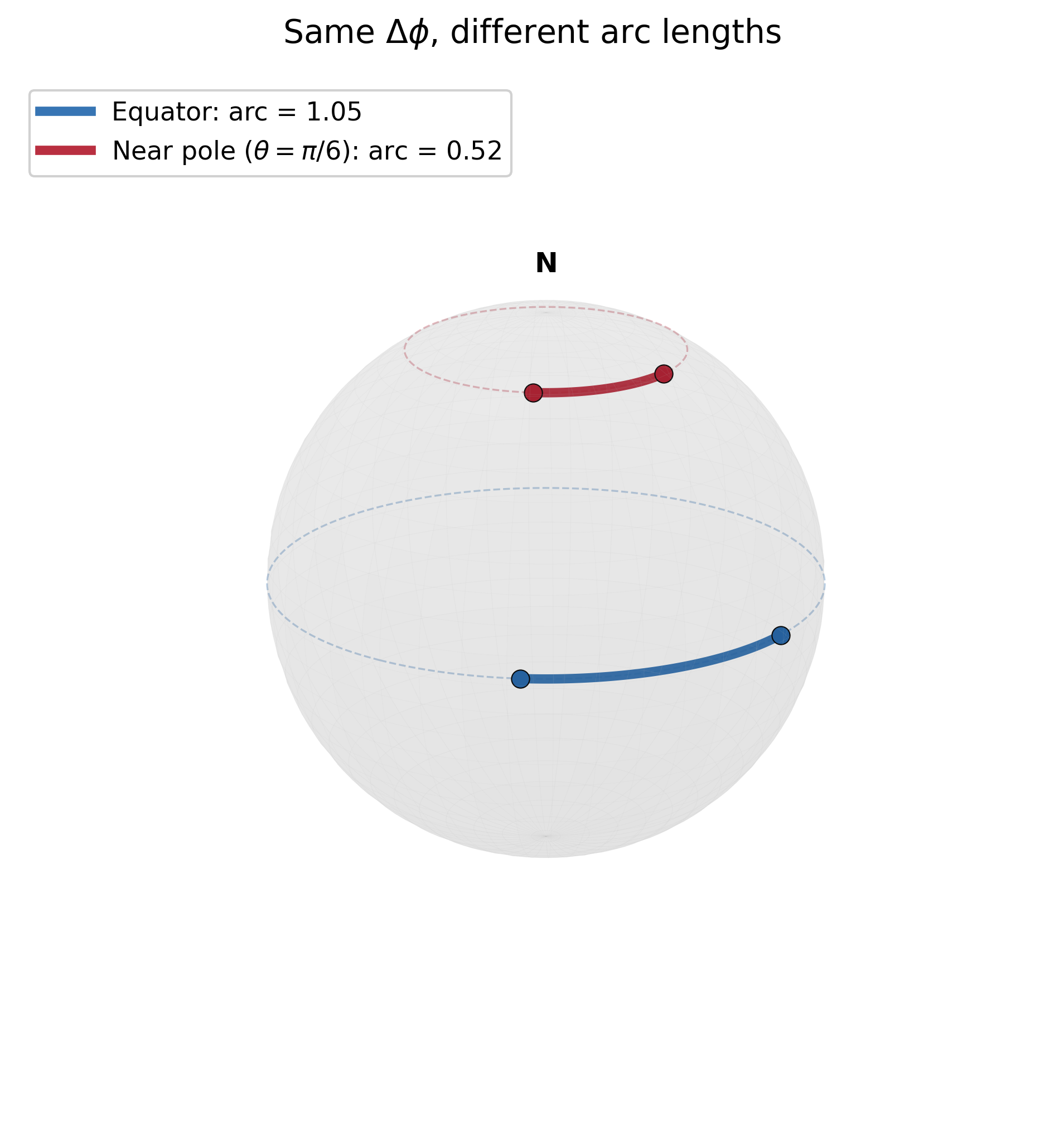
Consider the unit 2-sphere, parameterized by the usual spherical coordinates $(\theta, \phi)$. $\theta$ is the polar angle (co-latitude), ranging from $0$ to $\pi$. $\phi$ is the azimuthal angle (longitude), ranging from $0$ to $2\pi$. The metric tensor for the 2-sphere is:

\[g_{\mu \nu} = \begin{pmatrix} 1 & 0 \\ 0 & \sin^2\theta \end{pmatrix}\]

And if we displace by $(\Delta \theta, \Delta \phi)$, we have:

\[\begin{align} ds^2 &= \begin{pmatrix} \Delta \theta & \Delta \phi \end{pmatrix} \begin{pmatrix} 1 & 0 \\ 0 & \sin^2\theta \end{pmatrix} \begin{pmatrix} \Delta \theta \\ \Delta \phi \end{pmatrix} \\ &= (\Delta \theta)^2 + \sin^2\theta\, (\Delta \phi)^2 \end{align}\]

Here we see that the sphere is fundamentally different from Euclidean space: a displacement of one unit in $\phi$ corresponds to different actual distances depending on your latitude. The reason is that the circles of latitude get smaller as you approach the poles. Near the equator, $\sin\theta$ is close to 1, so a unit of $\phi$ corresponds to nearly a full unit of arc length. Near the poles, $\sin\theta$ is close to 0, so the same unit of $\phi$ corresponds to a much smaller arc length.

This is the role of the metric tensor: given a coordinate system that we use to represent our space, the metric tensor tells you, for a given displacement in those coordinates, how much actual distance is being traversed. The metric tensor encodes the geometry of our space.

The metric tensor also acts as an index-lowering operator, defining the inner product on each tangent space. You can’t actually directly dot two vectors together—to take the inner product, you must first lower one of the vectors into a covector using the metric tensor and then contract:

\[\vec{u} \cdot \vec{v} = u^\mu (g_{\mu\nu}\, v^\nu)\]

The metric tensor gives the canonical correspondence between vectors and covectors: for a given vector, its associated covector is the linear map defined by dotting that vector with other vectors. Conversely, for a given covector, its associated vector is the one that implicitly defines that linear map.

In the context of optimization, choosing a preconditioner $P$ is equivalent to choosing a metric on our parameter space. The preconditioned gradient descent update:

\[\theta_{t+1} = \theta_t - \eta\, P^{-1} \nabla L\]

is the Riemannian gradient descent with respect to the metric $P$.

Evidently, this helps motivate why the convention is $P^{-1}$ rather than $P$: the preconditioner $P$ is the metric tensor $g_{\mu\nu}$ and its inverse $P^{-1}$ is the inverse metric tensor $g^{\mu \nu}$.

Different preconditioners correspond to different geometries on parameter space. Each choice of preconditioner defines a different notion of “steepest descent”—the direction that decreases the loss fastest per unit distance.

Some Examples of Pre-Conditioners

Newton’s method is the prototypical second-order method. The preconditioner is the Hessian $\nabla^2 L$, so the update rule is:

\[\theta_{t+1} = \theta_t - [\nabla^2 L(\theta_t)]^{-1} \nabla L(\theta_t)\]

The key property of Newton’s method is that it solves quadratic losses in exactly one step. For a quadratic loss, no matter where you start, a single Newton step takes you directly to the minimum. Consider the quadratic loss:

\[L(\theta) = \frac{1}{2}(\theta - \theta^{*})^T H (\theta - \theta^{*})\]

The gradient is given as:

\[\nabla L(\theta) = H(\theta - \theta^*)\]

From any point $\theta_t$, the Newton update gives us:

\[\begin{align} \theta_{t+1} &= \theta_t -H^{-1}\nabla L(\theta_t) \\ &= \theta_t -H^{-1} [H(\theta_t - \theta^*)] \\ &= \theta_t -(\theta_t - \theta^*) \\ &= \theta^* \end{align}\]

which lands exactly at the minimum in one step.

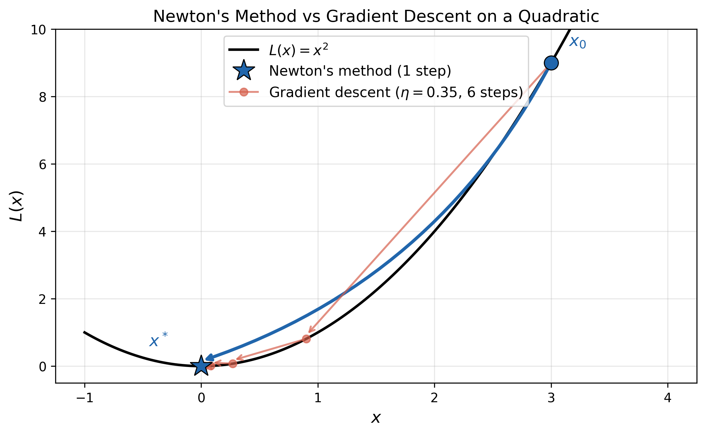
For a non-quadratic loss, Newton’s method works by locally approximating the loss as a quadratic by Taylor expanding around the current point $\theta_t$:

\[L(\theta) \approx L(\theta_t) + \nabla L(\theta_t)^T(\theta - \theta_t) + \frac{1}{2}(\theta - \theta_t)^T \nabla^2 L(\theta_t)(\theta - \theta_t)\]

This is a quadratic in $\theta$, so Newton’s method on the original loss is equivalent to exactly solving this local quadratic approximation. The better the quadratic approximation is to fitting the loss, the better Newton’s method works.

If we interpret the preconditioner as a metric tensor, then Newton’s method treats the Hessian $\nabla^2 L$ as a metric on the space of parameters. By doing so, it’s endowing the parameter space with a geometry directly tied to the loss: directions where the loss changes more quickly count as more “distance”.

In directions where the loss curves sharply, a small coordinate displacement already moves you a lot along the loss surface, so the inverse-Hessian shrinks your step. In directions where the loss is nearly flat, you can afford larger steps, so the inverse-Hessian stretches them out. The result is that Newton’s method perfectly adapts step sizes to curvature in every direction simultaneously.

Unfortunately, in machine learning, Newton’s method is rarely used: computing the Hessian for a large neural network is prohibitively expensive both computationally and in terms of storage. If the network has $p$ parameters, the Hessian is a $p \times p$ matrix—and for modern networks, $p$ can be in the billions. Computing, storing, and inverting a matrix of that size is out of the question. This is what motivates the search for preconditioners that capture some of the benefits of second-order information without the full cost.

Another example of a pre-conditioned gradient descent method is the natural gradient. The natural gradient takes a different perspective on what the “right” metric should be compared to Newton’s method. Rather than asking “how much does the loss curve in this direction?”, it asks: “how much does the function represented by the network change in this direction?”

Neural network architectures represent parametric families of functions $f(x;\theta)$. While we represent the parameters as a point in $\mathbb{R}^p$, Euclidean distance in parameter space is not particularly meaningful. A small displacement in one direction might barely change the network’s output, while the same-sized displacement in another direction might change it dramatically. What we want is a metric that reflects how much the network’s behavior actually changes—and that is exactly what the Fisher information matrix provides.

The Fisher information is properly defined not for families of functions, but for families of probability distributions. To bridge the gap, we can reinterpret the network as implicitly encoding a probabilistic model. For a network trained with MSE loss, we can treat it as specifying the mean of a Gaussian with fixed variance $\sigma^2$:

\[p(y \mid x;\, \theta) = \frac{1}{\sqrt{2\pi\sigma^2}}\exp\!\left(-\frac{(y - f(x;\,\theta))^2}{2\sigma^2}\right)\]

This is a modeling choice, but a mild one: since $\sigma^2$ is a fixed scalar, it only rescales the resulting metric without changing its geometry in any essential way. The Fisher information matrix is then:

\[F_{ij}(\theta) = \mathbb{E}_{(x,y) \sim p(\cdot\,;\,\theta)}\!\left[\frac{\partial \log p(y \mid x;\,\theta)}{\partial \theta^i}\,\frac{\partial \log p(y \mid x;\,\theta)}{\partial \theta^j}\right]\]

The Fisher information measures how much the output distribution changes per unit change in the parameters. More precisely, it is the metric tensor on the statistical manifold—the space of probability distributions parameterized by $\theta$. The Fisher Information arises naturally as the Hessian of the KL divergence between nearby distributions:

\[D_{\mathrm{KL}}(p_\theta \| p_{\theta + d\theta}) \approx \frac{1}{2}\, d\theta^T\, F(\theta)\, d\theta\]

The natural gradient update is:

\[\theta_{t+1} = \theta_t - \eta\, F^{-1}(\theta_t)\, \nabla_\theta L\]

The natural gradient $F^{-1}\nabla_\theta L$ is the steepest descent direction measured not in parameter-space distance, but in KL-divergence distance. It is the direction that decreases the loss fastest per unit change in the represented function.

A key property of the natural gradient is reparameterization invariance. If you change coordinates $\theta \to \phi(\theta)$, the natural gradient update moves to the same point regardless of the parameterization. This is why it is called the “natural” gradient: it is the gradient that is natural (intrinsic) to the space of distributions, not tied to any particular parameterization.

In practice, the Fisher information matrix is also too expensive to compute for large networks (it is the same size as the Hessian: $p \times p$).

In terms of actual machine learning optimization algorithms used in practice, one of the most influential is RMSprop. RMSprop maintains a running average of the squared gradients for each parameter:

\[v_t = \beta\, v_{t-1} + (1-\beta)\, g_t^{\odot 2}\]

where $g_t = \nabla_\theta L$ is the gradient at step $t$ and $\odot 2$ denotes the elementwise square. The parameters are then updated by dividing the gradient by the square root of this running average:

\[\theta_{t+1} = \theta_t - \frac{\eta}{\sqrt{v_t} + \epsilon}\, \nabla_\theta L\]

where $\epsilon$ is a small constant for numerical stability.

The preconditioner $\sqrt{v_t}$ is playing the role of a diagonal metric tensor on parameter space:

\[g_{ij} = \sqrt{v_i} \,\delta_{ij}\]

Dividing by $\sqrt{v}$ is applying the inverse metric $g^{-1}$ to convert the gradient covector into an update vector. But why would this be a good choice of metric?

The key insight is that the squared gradient in a given direction carries information about the curvature in that direction. To see why, consider a simple diagonal quadratic loss with two parameters:

\[L(\theta) = \frac{1}{2}(a\,\theta_1^2 + b\,\theta_2^2)\]

where $a \gg b$, so the loss curves much more sharply in the $\theta_1$ direction. The gradient is $(a\theta_1,\, b\theta_2)$, and the squared gradients are $(a\theta_1)^2$ and $(b\theta_2)^2$. The steep direction produces larger squared gradients, and the flat direction produces smaller ones. So RMSprop’s running average $v_i \approx \mathbb{E}[(\partial_i L)^2]$ is larger for high-curvature directions and smaller for low-curvature directions—which is exactly the information needed to adapt step sizes. Dividing by $\sqrt{v_i}$ shrinks the step in the steep direction and stretches it in the flat direction.

This is not exactly Newton’s method: RMSprop only adapts per-parameter (a diagonal approximation), and it uses the square root of the accumulated squared gradients rather than the full Hessian inverse. But it captures the essential adaptive behavior—parameters with large curvature get smaller updates, and parameters with small curvature get larger updates—cheaply and without ever computing second derivatives.