If you have a particle in a potential field $V$, the force tells you the direction the particle will move. The force points “downhill”: the direction in which the particle’s potential decreases most rapidly per unit distance. Mathematically, the force is the negative gradient of the potential:

\[F = -\nabla V\]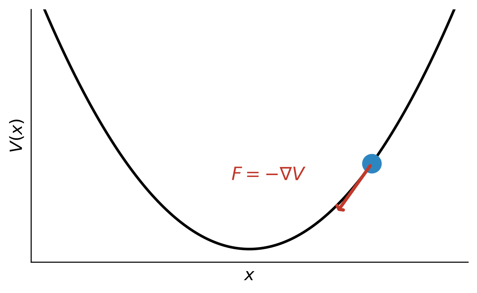

A ball on a potential landscape with force pointing downhill

Similarly, you can define a potential functional $\mathcal{V}$ that takes a probability distribution $\mu$ as input and returns a number: $\mathcal{V}: \mathcal{P}(\mathbb{R}^d) \rightarrow \mathbb{R}$.

We would like to understand how the distribution $\mu_t$ evolves over time to minimize this functional. But how do we define “downhill” for probability distributions? The notion of steepest descent requires a metric: the gradient is the direction that decreases the functional fastest per unit distance. In Euclidean space, we can default to the Euclidean metric. But for functionals on measures, there is no single canonical metric—and different metrics give rise to genuinely different gradients.

The most obvious choice is to treat the density as an infinite-dimensional vector whose dimensions are indexed by the base space $\mathbb{R}^d$. The inner product on this space corresponds to the pointwise product of functions integrated with respect to the Lebesgue measure. And the associated metric is the one induced by this inner product:

\[d_{L^{2}}(\mu, \nu) = \langle \mu - \nu, \mu - \nu \rangle = \int |\mu(x) - \nu(x)|^2 \, dx\]

Using this $L^2$ metric, “downhill” in measure space is given by the first variation of the functional $\mathcal{V}$.

But this choice treats the base space as merely an index set—it ignores its topology. Unlike in the finite-dimensional case, there is structure relating the dimensions of our vector space: some dimensions are closer to each other than others. Physically, we expect the correct dynamics to transport mass locally, as if the measure were made of tiny particles being pushed around.

A more principled choice is the Wasserstein-2 metric, which measures how the far mass must physically travel:

\[W_2^2(\mu, \nu) = \inf_{\gamma \in \Gamma(\mu, \nu)} \int \|x - y\|^2 \, \gamma(dx, dy)\]

The Wasserstein metric lifts the Euclidean metric to the space of measures: when the two measures are point masses, it directly coincides with the Euclidean metric. Using this metric to define “downhill” gives rise to the Wasserstein gradient.

The First Variation

Perhaps the simplest approach to defining a metric on the space of probability measures is the $L^2$ metric.

We can represent a measure by its density $\mu(x)$ and treat the density as an infinite-dimensional vector, with each spatial location $x \in \mathbb{R}^d$ indexing a different component. A useful intuition: integrating a function against a density is just an infinite-dimensional dot product. When we integrate a function against a density, we multiply the two “vectors” $f(x)$ and $\mu(x)$ componentwise and sum—which is exactly what a dot product does. This gives rise to the $L^2$ inner product:

\[\langle f, g \rangle_{L^2} = \int f(x) \, g(x) \, dx\]

which induces the metric:

\[d_{L^{2}}(\mu, \nu) = \int |\mu(x) - \nu(x)|^2 \, dx\]

The gradient of a functional $\mathcal{V}$ with respect to this inner product is the first variation $\frac{\delta \mathcal{V}}{\delta \mu}$. It’s defined by:

\[\frac{d}{d\varepsilon}\bigg|_{\varepsilon=0} \mathcal{V}(\mu + \varepsilon \chi) = \int \frac{\delta \mathcal{V}}{\delta \mu}(x) \, d\chi(x) = \left\langle \frac{\delta \mathcal{V}}{\delta \mu}, \chi \right\rangle_{L^2}\]

This is exactly analogous to the finite-dimensional case: the first variation is the object you “dot” with a measure perturbation $\chi$ to get the change in $\mathcal{V}$, just as the gradient $\nabla V$ is the vector you dot with a displacement $dx$ to get the change in $V$.

As a quick example, consider the potential energy functional $\mathcal{V}(\mu) = \int V \, d\mu$. Recall that for finite-dimensional vectors, $\frac{\partial}{\partial x_i}(a \cdot x) = a_i$. The first variation of the potential energy functional can be found by an analogous computation:

\[\begin{align} \frac{\delta \mathcal{V}}{\delta \mu(x)} &= \frac{\delta}{\delta \mu(x)} \int V(x') \, \mu(x') \, dx' \\ &= \int V(x') \, \frac{\delta \mu(x')}{\delta \mu(x)} \, dx' \\ &= \int V(x') \, \delta(x' - x) \, dx' \\ &= V(x) \end{align}\]

This makes sense: adding a unit point mass at $x$ increases the value of the functional by $V(x)$.

However, there are problems with the $L^2$ metric. To see why it’s the wrong choice of metric, consider the functional $\mathcal{V}(\mu) = \int x^2 \, d\mu$. The first variation is $x^2$, so the $L^2$ gradient flow is:

\[\partial_t \mu = - \frac{\delta \mathcal{V}}{\delta \mu} = -x^2\]

This suffers from an immediate problem: the perturbation doesn’t integrate to zero, so mass isn’t conserved. One might try to fix mass conservation by projecting onto zero-mean perturbations: $\tilde{\chi}(x) = -x^2 + \langle x^2 \rangle_\mu$.

But there is an even deeper problem: even when your current distribution $\mu$ is compactly supported, $\tilde{\chi}(x)$ is nonzero almost everywhere—which implies that density is simultaneously created and destroyed at points arbitrarily far from the current mass. The dynamics are non-local: mass teleports rather than flows.

The root issue is that the $L^2$ metric compares density values at each point independently, with no regard for where those points are in space. It treats the base space $\mathbb{R}^d$ as an unstructured index set. We need a metric that respects the geometry of the base space.

The Wasserstein Gradient

We insist on two physically-motivated requirements for the evolution of $\mu_t$:

Mass conservation. The total probability mass $\int \mu_t \, dx$ should remain constant.
Locality. Mass should move continuously through space. If the density decreases somewhere, it’s because mass flowed out to neighboring regions—not because it teleported.

Both requirements are satisfied if the measure evolves according to a continuity equation:

\[\partial_t \mu_t = -\nabla \cdot (\mu_t \, v_t)\]

where $v_t : \mathbb{R}^d \to \mathbb{R}^d$ is a velocity field. We can imagine the measure as composed of tiny indivisible particles—and $v_t(x)$ prescribes how the particle at position $x$ moves at time $t$.

Continuity equations appear throughout physics whenever a quantity obeys a local conservation law: energy conservation in classical mechanics, charge conservation in electrodynamics, and mass conservation in fluid dynamics.

Here, the conserved quantity is probability. If we integrate both sides of the continuity equation over all space:

\[\frac{d}{dt} \int \mu_t \, dx = -\int \nabla \cdot (\mu_t \, v_t) \, dx = 0\]

by the divergence theorem (assuming $\mu_t v_t$ decays at infinity). And locality is built in because the continuity equation is a local PDE—the density at a point changes only due to flux from nearby regions of space.

We want the velocity field that decreases $\mathcal{V}(\mu_t)$ as fast as possible. Recall that given a perturbation to the density, we can find the change in $\mathcal{V}$ by “dotting” the perturbation with the first variation. If we invoke the continuity equation for our density perturbation, we can derive an expression for how $\mathcal{V}$ changes along the flow generated by $v_t$:

\[\begin{align} \frac{d}{dt} \mathcal{V}(\mu_t) &= \int \frac{\delta \mathcal{V}}{\delta \mu} \, \partial_t \mu_t \\ &= -\int \frac{\delta \mathcal{V}}{\delta \mu} \, \nabla \cdot (\mu_t \, v_t) \\ &= \int \left\langle \nabla \frac{\delta \mathcal{V}}{\delta \mu}, \, v_t \right\rangle d\mu_t \end{align}\]

where the last step follows from integration by parts.

Just as the first variation is the object you dot density perturbations against (under the $L^2$ inner product) to get changes in $\mathcal{V}$, $\nabla \frac{\delta \mathcal{V}}{\delta \mu}$ is the object you dot velocity fields against (under the $L^2(\mu)$ inner product) to get changes in $\mathcal{V}$. It follows that the velocity field of steepest ascent is given by:

\[v_t = \nabla \frac{\delta \mathcal{V}}{\delta \mu}\]

This velocity field is the Wasserstein gradient of $\mathcal{V}$ at $\mu$:

\[\nabla_W \mathcal{V}(\mu) = \nabla \frac{\delta \mathcal{V}}{\delta \mu}\]

A key conceptual point: the Wasserstein gradient is not a “vector field in the space of measures”—it’s a vector field in the base space $\mathbb{R}^d$. This is a genuinely new feature of optimization over the space of probability measures with no direct analogue in the finite-dimensional Euclidean case. The Wasserstein gradient exploits the fact that our infinite-dimensional vector has an index set—the points $x \in \mathbb{R}^d$—that has its own differential structure. In finite dimensions, the index set $\{1, \ldots, d\}$ is discrete, so there is no spatial gradient to take.

We derived the Wasserstein gradient from the continuity equation without ever mentioning optimal transport. But we implicitly chose a geometry on the space of measures when we measured the “size” of a velocity field using $\int |v_t|^2 \, d\mu_t$—the $L^2(\mu_t)$ norm. Why does this choice of inner product on the space of vector fields correspond to endowing the space of probability measures with the Wasserstein-2 metric?

The answer comes from the Benamou–Brenier formula. Define the distance between two measures $\mu_0$ and $\mu_1$ as the minimum “kinetic energy” needed to transport one into the other via the continuity equation:

\[W_2^2(\mu_0, \mu_1) = \inf_{(\mu_t, v_t)} \int_0^1 \int \|v_t(x)\|^2 \, d\mu_t(x) \, dt\]

where the infimum is over all paths $(\mu_t, v_t)$ satisfying the continuity equation $\partial_t \mu_t = -\nabla \cdot (\mu_t v_t)$ with the correct endpoints. One of the most famous results in all of optimal transport theory is that this distance metric is equivalent to the Wasserstein-2 distance:

\[W_2^2(\mu, \nu) = \inf_{\gamma \in \Gamma(\mu, \nu)} \int \|x - y\|^2 \, d\gamma(x, y)\]

where $\Gamma(\mu, \nu)$ is the set of all couplings of $\mu$ and $\nu$.

The Benamou–Brenier formula makes the connection transparent: the $W_2$ metric is the one that arises naturally when you restrict evolution to the continuity equation and measure the cost of a velocity field by its $L^2(\mu)$ kinetic energy.

Some Worked Examples

Once again, consider the potential energy functional:

\[\mathcal{V}(\mu) = \int V \, d\mu\]

The first variation is $V(x)$, so the Wasserstein gradient is $\nabla V$—the force field. If we think of the measure as constituted of particles, each particle works independently to minimize the potential of the measure. There are no interaction forces between particles. This is because the functional is linear in the measure: each particle’s contribution to the potential energy is independent of where all the other particles are.

Now consider the entropy functional:

\[\mathcal{S}(\mu) = -\int \mu(x) \log \mu(x) \, dx\]

The first variation is $-\log \mu(x) - 1$, and the Wasserstein gradient is $-\nabla \log \mu$.

The first variation makes sense: entropy is higher when there is greater uncertainty—when the measure is more spread out. If we want to increase the entropy, it’s most impactful to allocate measure to where $\mu(x)$ is currently the smallest (which is where $-\log \mu(x)$ is largest).

The Wasserstein gradient translates this into particle dynamics: each particle moves down the gradient of the log-density, away from regions of high concentration. From a physical perspective, the entropic force manifests as a repulsive force between particles. This is because the entropy functional $\mathcal{S}$ is nonlinear in the measure—we now have a system where particles interact with each other.

If we plug the Wasserstein gradient of the entropy into the continuity equation, we get:

\[\partial_t \mu_t = \nabla \cdot (\mu_t \, \nabla \log \mu_t) = \Delta \mu_t\]

This is simply the heat equation. Diffusion, usually viewed as a local process driven by intermolecular collisions, can equivalently be viewed as the distribution itself performing gradient flow on the entropy functional.

Now consider the free energy functional which is a combination of the potential energy functional and the entropy functional:

\[\begin{align} \mathcal{F}(\mu) &= \mathcal{V} - \mathcal{S} \\ &= \int \mu(x) \left[ V(x) + \log \mu(x) \right] dx \end{align}\]

Because the Wasserstein gradient is linear, we can combine our two previous results:

\[\nabla_W \mathcal{F} = \nabla V + \nabla \log \mu\]

And plugging the Wasserstein gradient into the continuity equation, we get:

\[\begin{align} \partial_t \mu_t &= -\nabla \cdot (\mu_t \, \nabla V) - \nabla \cdot (\mu_t \, \nabla \log \mu_t) \\ &= -\nabla \cdot (\mu_t \, \nabla V) + \Delta \mu_t \end{align}\]

This is the Fokker-Planck equation. The drift term comes from the potential, and the diffusion term comes from entropy. Fokker-Planck is Wasserstein gradient flow of the free energy—this is the celebrated result of Jordan, Kinderlehrer, and Otto.