Neural Tangent Kernel Explained

While neural networks learn features—with the accompanying nonlinear parametrization and non-convex loss landscapes—it turns out that when the final trained model has parameter values very close to the initial values, we can approximate the training dynamics with a linear model. And while the loss landscape is formally non-convex, because the training dynamics stays in a small neighborhood of the initialization, the landscape is effectively convex. No meaningful feature learning occurs.

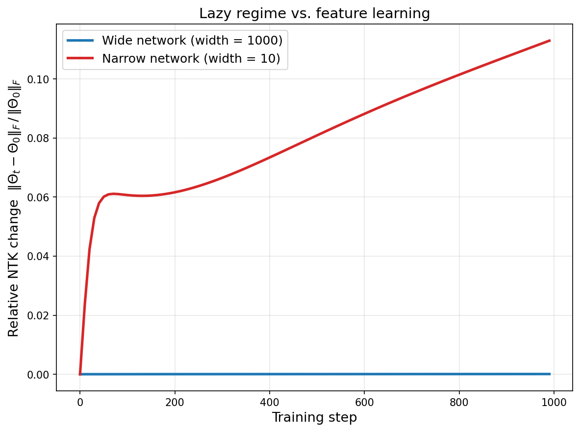
When the parameters stay close to their initialization during training, we say we are in the lazy training regime. And the object that governs lazy training is the neural tangent kernel (NTK). The NTK tells us how a neural network learns to fit the training data when its features don’t change—and by contrast, it highlights that feature learning is the essential ingredient that makes deep learning more than kernel regression.

Linearization Near Initialization

Consider a neural network $f(x; \theta)$ initialized at some $\theta_0$. In a neighborhood around the initial parameters, we can approximate the network by Taylor expanding:

\[f(x; \theta) \approx f(x; \theta_0) + \nabla_\theta f(x; \theta_0) \cdot (\theta - \theta_0)\]

The right-hand side is linear in $\theta$: the term $f(x; \theta_0)$ is a constant (determined by initialization), and $\nabla_\theta f(x; \theta_0)$ is a fixed vector (also determined by initialization) that is independent of the current value of $\theta$. We can define the following as relevant features:

\[\phi_i(x) = \frac{\partial f}{\partial \theta_i}\bigg|_{\theta_0}\]

Let $p$ be the number of parameters in the network and $\Delta \theta$ be the difference between the current and initial parameter values. We then have:

\[f(x; \theta_0 + \Delta \theta) - f(x; \theta_0) \approx \sum_{i=1}^p \Delta \theta_i \, \phi_i(x)\]

If the loss has a global minimum such that this local expansion around initialization is valid, we are back in the familiar setting of linear regression—except now our features are the gradients of the network output with respect to each parameter, evaluated at initialization. A key difference from ordinary linear regression is that rather than choosing the feature map by hand, the features are random: the network architecture and random initialization jointly determine the feature map.

From Features to Kernels

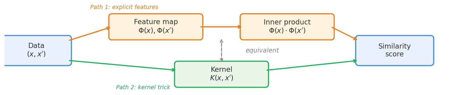
We’ve been speaking the language of features: functions of the input that capture how the network preprocesses the data. But there is an equivalent and complementary perspective: that of a kernel.

A kernel is a function that takes two input data points and returns a scalar measuring how similar they are. The feature map perspective and the kernel perspective are two different ways of looking at the same thing—how the model understands the structure of the input data. If you have a set of features, you can stack them into a vector:

\[\Phi(x) = \langle \phi_1(x), \phi_2(x), \ldots, \phi_p(x) \rangle\]

and define the kernel as the inner product of the feature vectors of two data points:

\[K(x, x') = \Phi(x) \cdot \Phi(x')\]

Conversely, if you know the kernel, you can (in principle) recover the feature map. This is the content of Mercer’s theorem: every positive definite kernel corresponds to an inner product in some feature space. The connection to kernel methods—a classical family of machine learning algorithms—is immediate: regression or classification using the kernel is equivalent to linear regression in that implicit feature space.

To make this concrete, let’s consider a couple example kernels.

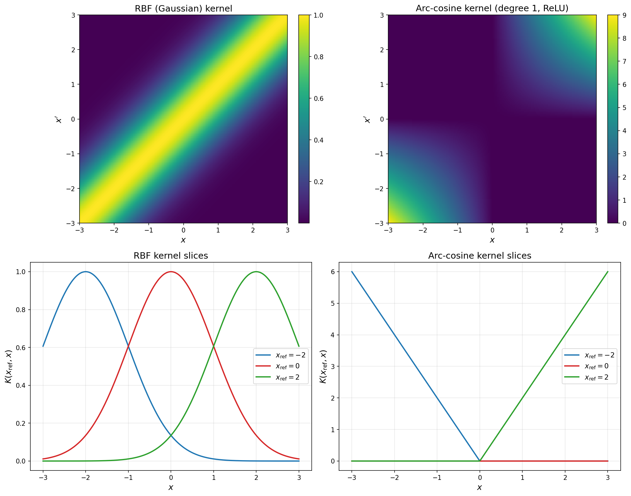
RBF (Gaussian) kernel. One of the most familiar kernels is the radial basis function kernel:

\[K(x, x') = \exp\!\left(-\frac{\|x - x'\|^2}{2\sigma^2}\right)\]

This kernel says that similarity decays with Euclidean distance—points close together are similar, points far apart are not. Despite being simple, the implicit feature map of the RBF kernel is infinite-dimensional. By Bochner’s theorem, the kernel can be expressed as:

\[K(x, x') = \int_{\mathbb{R}^d} p(\omega) \, e^{i\omega^\top x} \, e^{-i\omega^\top x'} \, d\omega\]

where $p(\omega)$ is a Gaussian distribution over frequency vectors $\omega$. The “features” are complex exponentials $e^{i\omega^\top x}$—one for every possible frequency—and the kernel is their inner product averaged over all frequencies, with higher frequencies downweighted by the Gaussian envelope.

Arc-cosine kernel. A less familiar but more relevant example is the arc-cosine kernel of degree 1:

\[K(x, x') = \frac{1}{\pi}\|x\|\,\|x'\|\!\left(\sin\alpha + (\pi - \alpha)\cos\alpha\right)\]

where $\alpha = \cos^{-1}(\hat{x} \cdot \hat{x}’)$ is the angle between the inputs. This is the kernel of a single hidden-layer ReLU network at initialization. Unlike the RBF kernel, the arc-cosine kernel is not a simple function of Euclidean distance: it depends on the magnitudes and angle of the inputs separately. Larger inputs produce larger kernel values, reflecting the scale-equivariance of ReLU ($\text{ReLU}(cx) = c\,\text{ReLU}(x)$ for $c > 0$). Holding magnitude constant, inputs pointing in similar directions (smaller $\alpha$) are more similar, since most random ReLU neurons that activate for one will also activate for the other. The kernel is always non-negative.

The Neural Tangent Kernel

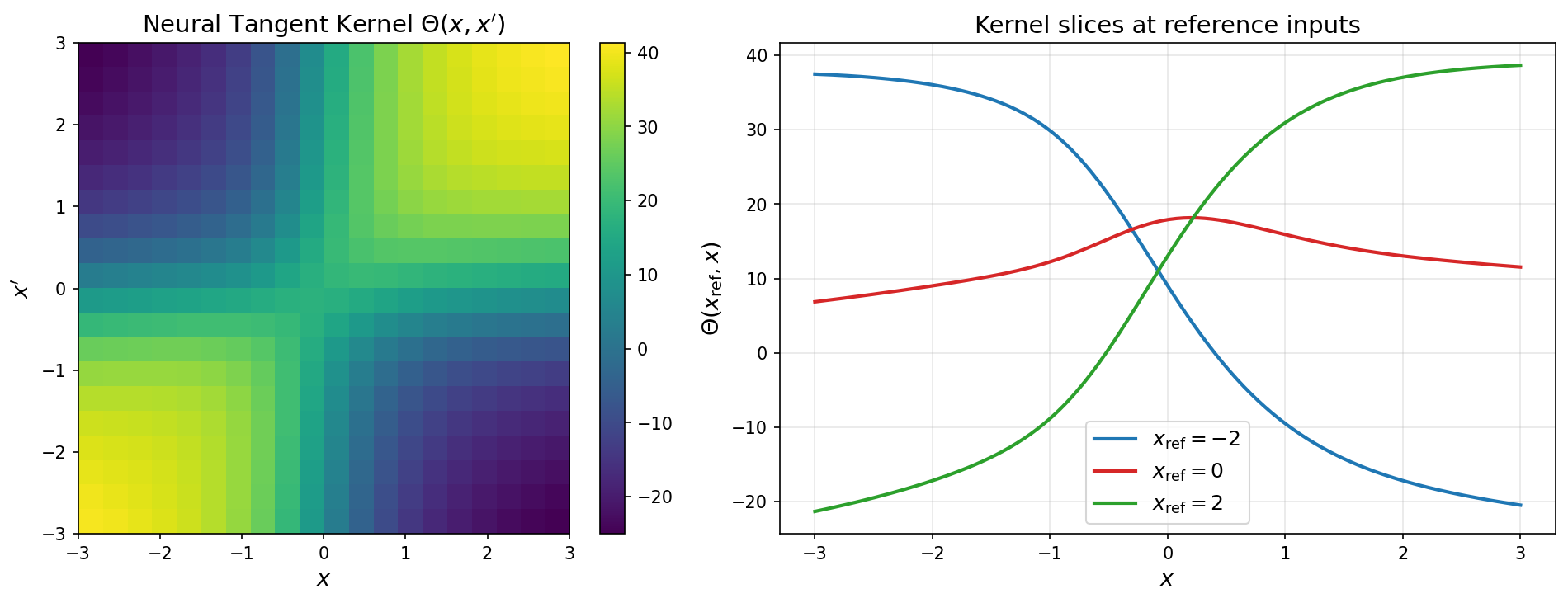
Recall that the gradient of the network output with respect to the parameters defines a $p$-dimensional vector of features. For any two inputs, we can define the neural tangent kernel:

\[\Theta(x, x') = \nabla_\theta f(x; \theta) \cdot \nabla_\theta f(x'; \theta)\]

The NTK is the kernel associated with the linearized network: just as the Jacobian defines the features of lazy training, the NTK is the corresponding kernel. (The name “neural tangent kernel” comes from the fact that it is derived from the tangent—the Jacobian—of the neural network.)

According to the NTK, two data points are similar if perturbing the parameters causes similar changes in the network’s output at those points. Note that similarity is based on the change in output under perturbation, not on the current output values. Two inputs can evaluate to the same output yet be dissimilar under the NTK, while two inputs with very different outputs can be similar. The NTK captures how the network “sees” the relationship between inputs through the lens of its parametrization.

A subtlety: the NTK treats all parameters symmetrically. The kernel $\Theta(x, x’)$ is invariant under rotations of the parameter space—it depends only on the inner product of gradients. This is the Euclidean geometry of the parameter space showing through. In more sophisticated treatments (e.g. natural gradient methods), one introduces a non-Euclidean geometry that weights different parameter directions differently.

The above defines the NTK for any two arbitrary inputs. But in practice, we work with the NTK as a matrix over our actual data points. For $n$ data points, we stack the gradients into the Jacobian matrix $J \in \mathbb{R}^{n \times p}$: each row is the gradient of the network output at one data point with respect to all $p$ parameters. The NTK matrix is then:

\[K = J J^\top\]

an $n \times n$ matrix whose entry $K_{ij}$ measures the similarity between data points $x_i$ and $x_j$.

If the NTK is just another reformulation of the feature map, why should we care about it?

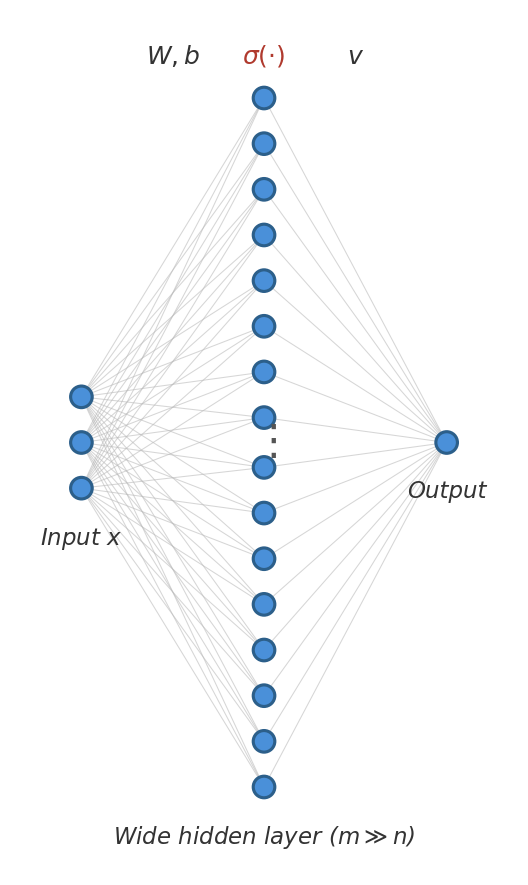
Because even though the feature map is random (due to random initialization), the NTK becomes deterministic in the infinite-width limit. To see why, note that the NTK is a sum over contributions from individual neurons:

\[\Theta(x, x') = \sum_{j=1}^{m} \nabla_{w_j} f(x) \cdot \nabla_{w_j} f(x')\]

Each term is random, but by the law of large numbers, this sum converges to its expectation as the width $m \to \infty$. The result is a fixed kernel that depends on the architecture but not on the particular random initialization. This is what makes the infinite-width limit of neural networks analytically tractable: the training dynamics reduce to kernel regression with a known, deterministic kernel.

The NTK framework was introduced by Jacot, Gabriel, and Hongler (2018) to provide a precise picture of how learning proceeds in the lazy regime. Under gradient descent with a fixed NTK, the network learns different components of the target function at different rates, governed by the eigenstructure of the NTK matrix $K$.

To see how, let $r \in \mathbb{R}^n$ be the residual vector: the vector whose $i$-th entry is the residual between the target $y_i$ and the network’s current output $f(x_i)$. Decomposing $r$ in the eigenbasis of $K$, each component decays exponentially at a rate proportional to the corresponding eigenvalue. Components aligned with the top eigenvectors of the NTK—the kernel principal components—are learned quickly. Components along small-eigenvalue directions are learned slowly.

Lazy Training Versus Rich Training

When is neural network training in the lazy regime? A couple factors are:

Width and parameterization. Let $m$ denote the width of the network (the number of neurons per layer). When a network has far more parameters than training examples, it can fit the data with very small parameter movements—and the linearization stays valid. Under the standard parameterization, weights are initialized at scale $O(1/\sqrt{m})$, so each neuron contributes $O(1/\sqrt{m})$ to the output. If each neuron’s weights are perturbed by $\delta$, the $m$ contributions add like independent random variables, producing a total output change of $O(\sqrt{m} \cdot \delta)$. To achieve an $O(1)$ change in the output, each parameter need only move by $O(1/\sqrt{m})$—vanishingly small as $m$ grows.

Learning rate relative to width. Whether a network learns features depends not just on width, but on how the learning rate scales with the width. In contrast with the standard parametrization, Yang and Hu introduced maximal update parameterization ($\mu$P), which rescales both the initialization and the per-layer learning rates so that each neuron’s weights move by $O(1)$ during training, regardless of width. Even without $\mu$P, a sufficiently large learning rate can push a finite-width network out of the lazy regime: large discrete gradient steps overshoot the region where the linearization is accurate, landing the parameters in a region where the features have changed.

We can define two distinct regimes of training.

In the lazy regime (NTK regime), parameters stay near initialization, features are fixed, optimization is effectively convex, and generalization performance depends on whether the random initial features happen to suit the task.

In the rich regime (feature-learning regime), parameters move substantially from initialization, features adapt to the data, and the network exploits structure that random features cannot capture.

Yesterday’s post argued that non-convexity is the price of feature learning. The lazy regime reveals a crucial subtlety: you can have a formally non-convex loss landscape that is effectively convex in the neighborhood of initialization—and in that case, no meaningful feature learning occurs. Non-convexity is necessary but not sufficient: feature learning requires that the optimization dynamics actually traverse the non-convex landscape, moving far enough from initialization that the features change. While non-convexity opens the door, it’s the dynamics that walk through it.