Non-Convexity As Feature Learning
In my review of Jared Kaplan’s machine learning notes, I made the point that neural network training loss functions are non-convex because the function represented by a given neural network is a nonlinear function of the parameters:
The loss function can actually be decomposed into two functions: the model output as a function of $\theta$ and the loss given the output:
\[\mathcal{L} = \ell \circ f\]where $\ell(\hat{y}) = |y - \hat{y}|^2$. Since $\ell$ is convex, the overall convexity of the loss depends entirely on the function $f$. In the case of linear regression, the predicted output is a linear function of the parameters. The composition of a linear function with a convex function is convex—that’s why the least-squares objective is convex. But in neural networks, $f$ is a non-linear function of the parameters $\theta$. The composition of a non-linear function with a convex function generically gives you a non-convex function. So the fact that neural networks can represent non-linear functions is intimately related to why they are so hard to train.
The final statement—that a neural network’s ability to represent nonlinear functions is intimately related to why it is so hard to train—wasn’t inaccurate, but it elided a subtle distinction: there is a difference between viewing the neural network as a function of the input data $x$ (with the parameters fixed) and as a function of the parameters $\theta$ (with the input fixed). Specifically, a neural network can be linear with respect to its parameters while still being a nonlinear function of the input.
Consider a simple example: a one-dimensional function expressed in the basis of polynomials.
\[f(x; \theta) = \sum_{k=0}^N \theta_k x^k\]This parametrization is nonlinear with respect to the input $x$, but linear with respect to the parameters $\theta$. It’s nonlinear with respect to $x$ because of the higher-order powers: $(x+y)^n \neq x^n + y^n$ unless $n = 1$. But it’s linear with respect to the parameters: if you have two functions in your space with parameter vectors $\theta$ and $\theta’$, the function with parameters $\theta + \theta’$ is the sum of the two functions: $f(x; \theta + \theta’) = f(x; \theta) + f(x; \theta’)$.
(In this case, this makes sense as the parameterization is familiar: we can identify the value of $\theta_k$ with the $k$-th derivative of the corresponding function divided by $k!$. And we know that derivatives are linear operations: the $k$-th derivative of the sum of two functions is the sum of their $k$-th derivatives.)
There are pros and cons to using a parametrization of your function space that is linear in the parameters. The pro is that because the model is linear in the parameters, our training objective is now convex. Consider a mean-squared error (MSE) loss where we attempt to find the function within our parametric family that best fits some target function $g$:
\[L(\theta) = \mathbb{E}_{x \sim \mathcal{D}}(g(x) - f(x;\theta))^2\]With the MSE loss, our problem becomes equivalent to solving a linear regression problem. The set of basis functions ${1, x, x^2, \ldots, x^N}$ plays the role of a feature map: a fixed set of nonlinear transformations of the input that we then combine linearly. Let $\phi_n$ denote the $n$-th feature in our feature map. Because the loss is convex, we can solve for the optimal parameters in closed form by taking the gradient of the loss and setting it to zero:
\[\nabla_\theta L(\theta) = -2\,\mathbb{E}[(g(x) - f(x;\theta))\,\nabla_\theta f(x;\theta)] = 0\]Since $f$ is linear in $\theta$, we have $\partial f / \partial \theta_n = \phi_n(x)$. So at the optimum $\theta^{\ast}$, for each component $\theta_n^{\ast}$, we get an equation of the form:
\[\mathbb{E}[g(x)\,\phi_n(x)] = \mathbb{E}[f(x;\theta^{\ast})\,\phi_n(x)]\]This has a nice geometric interpretation: the projection of the fitted function $f(x; \theta^{\ast})$ onto each feature equals the projection of the target function $g(x)$ onto that feature, where the “inner product” is the expectation of the pointwise product with respect to the data distribution.
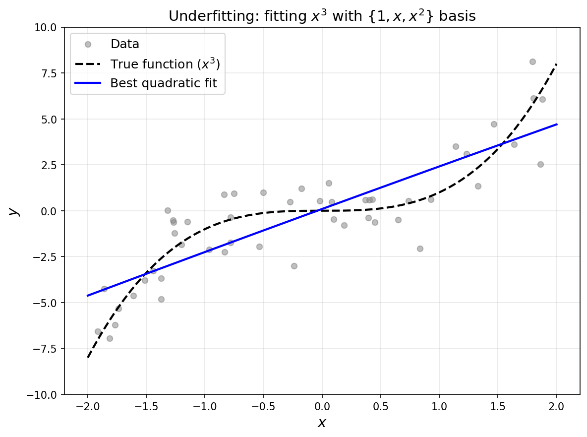
The con associated with a linear parametrization is that the features are fixed before training begins. If the target function has structure that isn’t captured by your chosen basis, you have no way to recover it. For example, if we are working in the polynomial basis ${1, x, x^2, \ldots, x^N}$ and the true function is $x^{N+1}$, we would have no way to fit it—we are stuck with the lower-order polynomials.
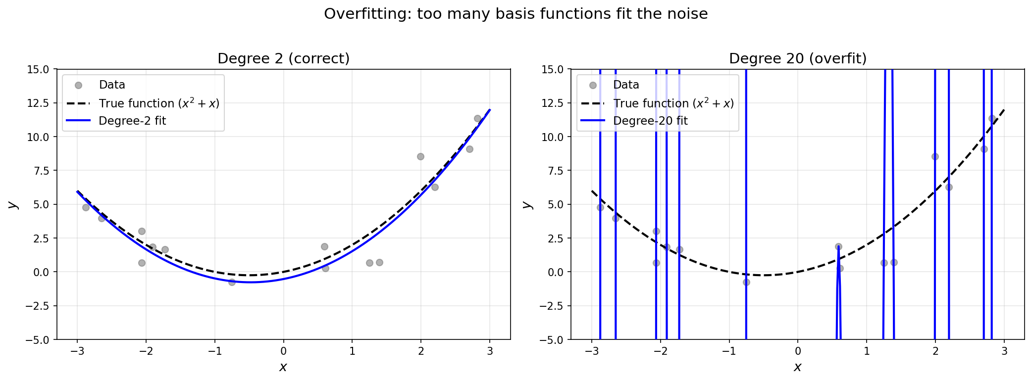
Why not just add more basis functions—one for each polynomial up to some very high degree? The problem is noise and finite samples. With a large basis, if we naively choose the function with the smallest training error, we end up fitting the noise rather than the underlying signal. And our overarching goal is not to perfectly fit the training data, but to generalize to the true underlying distribution.
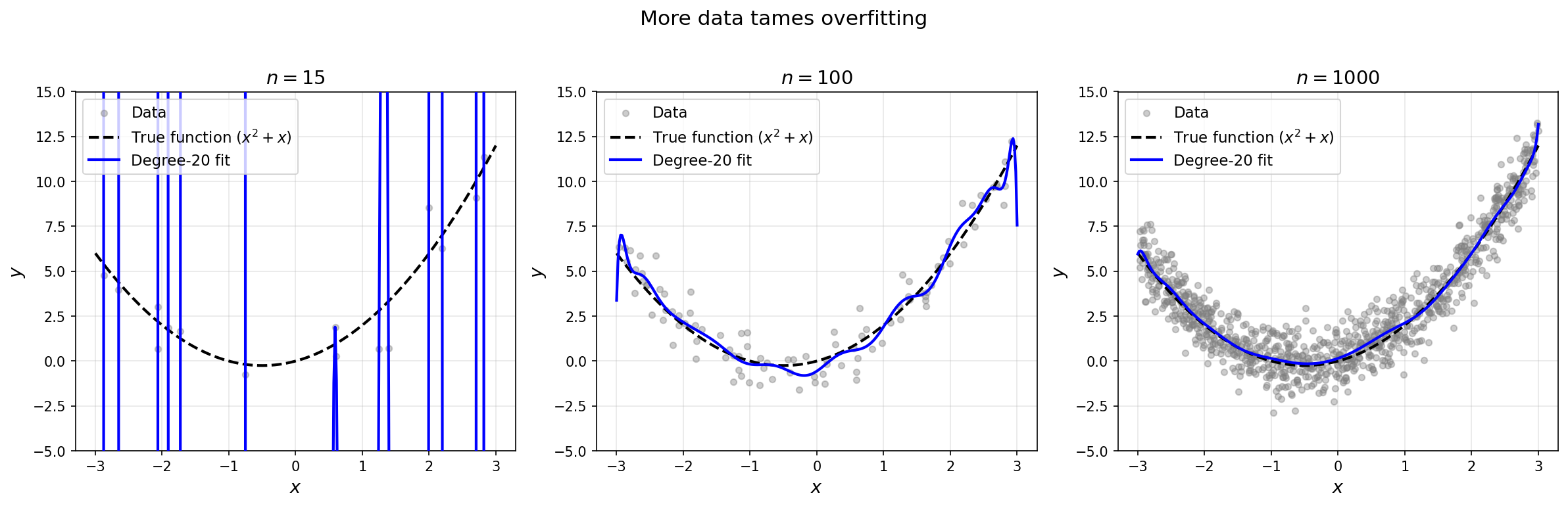
Note that if we were to collect a lot more data, this problem would go away: even with far more basis functions than we need, enough data would overwhelm the noise and the fit would converge to the true function.
This is the bias-variance tradeoff. A large set of features gives us low bias: in the limit of infinite data, we can represent any function in the span of the basis. But it comes with high variance: when working with finite samples, the fit is incredibly sensitive to noise. A smaller feature set gives us low variance: the fit is robust across different realizations of the noise. But small feature sets suffer from asymptotic bias: if the true function lies outside the span, no amount of data will recover it. There is an inherent tension between the expressiveness of the function space and the stability of the fitting procedure—and this tension becomes increasingly severe in high dimensions.
To see why, consider extending the polynomial basis to $d$ input dimensions. The set of all monomials up to degree $k$ in $d$ variables has $\binom{d+k}{k}$ elements. Even for moderate $d$ and $k$, this is enormous: degree-4 polynomials in 100 variables give over 4 million basis functions. Say you want to fit a function that depends on only ten of these monomials—but importantly, you aren’t told ahead of time which ones they are. With a fixed basis, you either include too many features (and overfit) or too few (and underfit).
Neural networks sidestep this dilemma by learning their features from data. Many real-world target functions, while highly nonlinear, have low-dimensional structure: they depend on a small number of directions or combinations of the inputs, not on all $\binom{d+k}{k}$ monomials equally. A fixed basis cannot exploit this structure, but a neural network can adaptively discover the relevant directions during training. This achieves both low bias (the learned features can represent the target) and low variance (the effective number of features is small). Feature learning is how neural networks navigate the bias-variance tradeoff.
To make this concrete, consider a two-layer neural network: a neural network with an input layer, one hidden layer, and then an output.
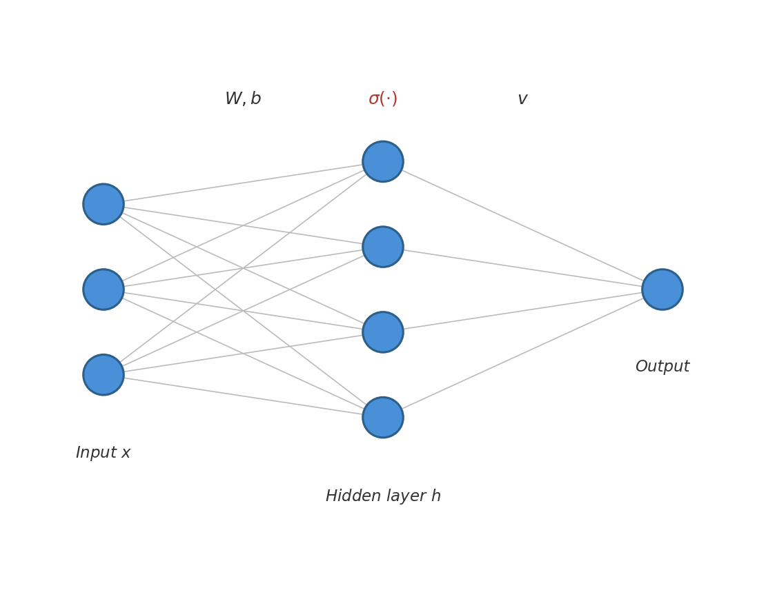
There are three steps to a two-layer neural network.
-
First, given the input data $x$, you apply a linear transformation $z = Wx + b$, where $W$ is a weight matrix and $b$ is a bias vector. Both $W$ and $b$ are learnable. The result $z$ is called the pre-activation.
-
Then you apply a nonlinear activation function $\sigma$ elementwise to get the hidden layer activations $h = \sigma(z) = \sigma(Wx + b)$. Common choices include ReLU (which zeroes out negative values and passes positive values through) and tanh (a sigmoidal function that smoothly maps inputs to the range $(-1, 1)$). The activation function is essential—the composition of linear transformations is itself linear, so you need the nonlinearity of the activation function for the network to be able to express nonlinear functions.
-
Finally, you project the vector of activations down to a single scalar using a learnable vector $v$. All together, the two-layer neural network is represented by the parametric family of functions:
The two-layer neural network can be interpreted in a manner similar to a linear parametrization. Let $w_i$ denote the $i$-th row of the weight matrix $W$ and $b_i$ the $i$-th component of the bias vector. Then each activation can be interpreted as computing the projection of the input $x$ onto $w_i$, shifting by $b_i$, and applying the nonlinear activation function. If we define $\phi_i(x) = \sigma(w_i \cdot x + b_i)$, then the final layer is just a linear combination of these features. But the key difference from ordinary linear regression is that the features $\phi_i(x)$ themselves depend on the learnable parameters $W$ and $b$. As a result, even though the model is linear in $v$ with the other parameters held fixed, it is nonlinear in the full parameter set $(W, b, v)$—and this is what makes the loss landscape non-convex.
This generalizes to deeper networks. A multi-layer perceptron (MLP), also known as a feedforward neural network, is a composition of layers: each layer applies a linear transformation (a weight matrix and bias vector) followed by a nonlinear activation function.
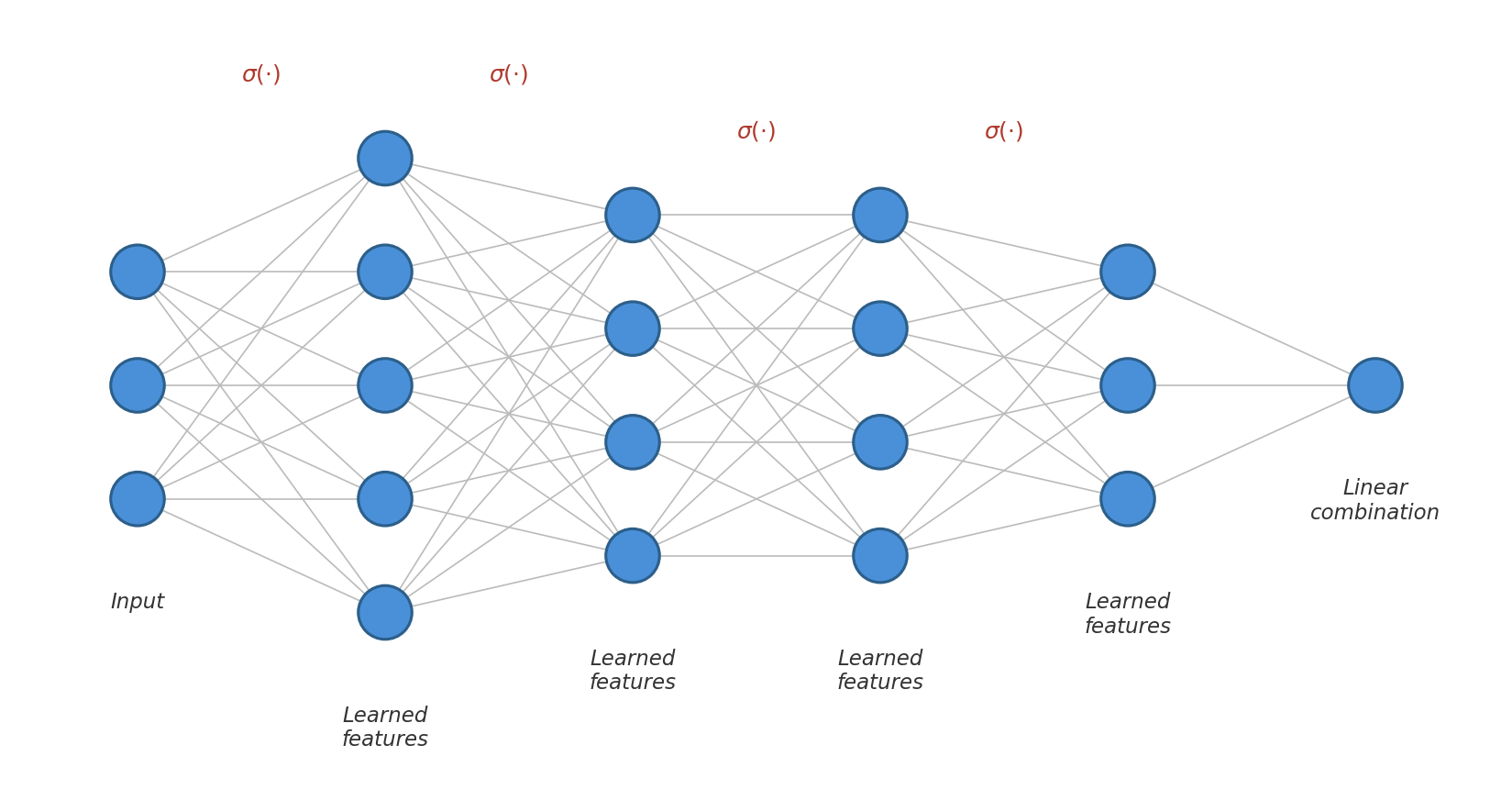
In an $N$-layer network, the first $N-1$ layers learn a feature representation and the final layer linearly combines those features. Depth compounds the nonlinearities, allowing the network to construct richer and more abstract features than a shallow network could. There is also a hierarchical interpretation: each layer learns features at a different level of abstraction. In an image classifier, for instance, early layers might learn to detect edges and textures, middle layers assemble these into parts of objects, and later layers recognize whole objects.
Feature learning is why neural network loss landscapes are non-convex. The power of neural networks comes from their ability to learn their own features, but this requires that the network be a nonlinear function of its parameters. The nonlinearity in the parameters causes the loss landscape to be non-convex. Non-convexity is the price of feature learning.