What is Edge of Stability?
In machine learning, we use data to train our models. We care not only about the final trained model, but also the training dynamics: the trajectory it takes in parameter space while learning from the data.
Over the course of training, the model adjusts its parameters to minimize the loss. We can visualize this process as navigating a loss landscape—a surface where height represents the loss value at each point in parameter space. This is why the field of optimization is relevant to describing neural network training dynamics.

A standard optimization algorithm is gradient descent. With gradient descent, we compute the gradient at the current parameter values and nudge the parameters in the opposite direction.
\[\theta_{t+1} = \theta_t - \eta \nabla L(\theta)\]where $\theta$ denotes the vector of parameters, $\eta$ denotes the step size, and $L$ denotes the loss function.
The gradient points toward the direction of steepest ascent, so moving against it leads us downhill. Furthermore, the magnitude of the gradient tells us how steep the loss landscape is at that point in parameter space.
However, we don’t just care about the steepness of the loss landscape, but also its curvature. This curvature is captured by the Hessian $\nabla^2 L$—the matrix of second derivatives of the loss—which tells us how the gradient itself changes as we move through parameter space.
In classic convex optimization, you want your step size to be small. If your step size is small, gradient descent will closely approximate gradient flow, and your iterates will roll smoothly downhill, settling near the closest local minimum. If the step size is too large relative to the curvature of the minimum you’re trying to reach, you won’t settle at the bottom—you’ll either oscillate back and forth or diverge entirely.
At what values of the step size will you converge? Consider a simple one-dimensional example: a quadratic potential of the form $\frac{a}{2}x^2$, which has a second derivative (curvature) of $a$.
-
For small step sizes ($\eta < \frac{1}{a}$), gradient descent approximates gradient flow and converges smoothly.
-
For medium step sizes ($\frac{1}{a} < \eta < \frac{2}{a}$), gradient descent bounces across the minimum but still converges.
-
For large step sizes ($\eta > \frac{2}{a}$), gradient descent diverges.
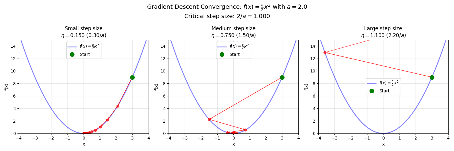
We can also invert this question: given a fixed step size $\eta$, what curvatures can we handle? The critical threshold is a curvature of $\frac{2}{\eta}$. Given a step size of $\eta$, this defines the maximum curvature for which gradient descent will converge.
In the quadratic examples above, the curvature is constant, so whether a step size leads to convergence is a global property.
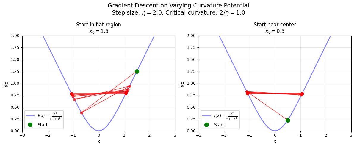
But consider a potential of the form $\frac{x^2}{\sqrt{1 + x^2}}$. In this potential, the curvature varies with distance from the origin. Far from the origin, it’s approximately flat. Near the origin, it behaves like a quadratic with curvature of 2. This varying curvature creates rich dynamics: if you start far from the minimum with a large step size, you might converge initially in the flatter regions, but as you approach the center where curvature increases, that same step size could cause divergence. Similarly, if you start close to the center, you’ll be repelled outward at first, before settling into a flatter region where you can converge. Regardless of your starting location, the dynamics will self-regulate—the effective curvature at your location will adjust to hover near the critical threshold of $\frac{2}{\eta}$.
Where things get particularly interesting is in the high-dimensional setting of neural networks. Different directions in parameter space can have vastly different curvatures. You might be oscillating wildly along one high-curvature direction while smoothly descending along another, flatter direction.
What theory predicts—and experiments confirm—is that directions with curvature exceeding $\frac{2}{\eta}$ will experience dynamics that reduce their curvature until it stabilizes near this critical value of $\frac{2}{\eta}$. This phenomenon is called the edge of stability: during training, the largest eigenvalue of the Hessian (called the sharpness) hovers around the threshold value of $\frac{2}{\eta}$ for extended periods of time.
The edge of stability reveals an important implicit bias of gradient descent: GD favors flatter minima over narrower minima.
In machine learning, we distinguish between explicit bias (regularization terms added directly to the loss function, like $L_2$ penalties) and implicit bias (the preferences induced by the optimization algorithm itself). While explicit biases are easier to analyze mathematically, the implicit biases of standard optimizers like SGD and Adam may be equally important for understanding why neural networks generalize well.