Statistical Optimal Transport Workshop 2025
A couple of months ago, Sinho told me that there would be a Statistical Optimal Transport Workshop hosted by Columbia University. It was excellent timing for another conference. While I’m still quite new to optimal transport, I’ve learned a lot over the past couple of months. Attending this conference would help to better contextualize the knowledge that I’ve acquired.
To recap: optimal transport is a subfield of probability theory which studies the best or “optimal” way to transform one probability distribution into another. It has its origins in the Monge problem: given a source mound of dirt and a target mound of dirt, how does one transform the source mound into the target mound while expending the least amount of energy?
More formally, in the Kantorovich formulation of the Monge problem, instead of finding a transport map that pushforwards $\mu$ into $\nu$, we look for the optimal coupling. A coupling of two probability distributions $\mu \in \mathcal{P}(\mathcal{X})$ and $\nu \in \mathcal{P}(\mathcal{Y})$ is a joint distribution $\gamma$ over $\mathcal{X} \times \mathcal{Y}$ where the $x$ and $y$ marginals are $\mu$ and $\nu$ respectively.
\[\mu(x) = \int_\mathcal{Y} dy \ \gamma(x,y), \quad \nu(y) = \int_\mathcal{X} dx\ \gamma(x,y)\]We denote $\Gamma(\mu, \nu) \subset \mathcal{P}(\mathcal{X} \times \mathcal{Y})$ to be the set of all couplings of $\mu$ and $\nu$. The transport cost is given by integrating the cost function with respect to the optimal coupling: the coupling that minimizes the expected cost.
\[\mathcal{C}(\mu, \nu) = \inf_{\gamma \in \Gamma(\mu, \nu)} \int c(x,y) \gamma(dx, dy)\]By using optimal transport, we can quantify the extent to which one probability distribution is “close” to another distribution. And for certain well-behaved cost functions, optimal transport defines a metric on the space of probability measures. The most commonly studied metric is the Wasserstein-2 metric, which uses the squared Euclidean distance as its cost function.
\[W_2(\mu, \nu) = \sqrt{\inf_{\gamma \in \Gamma(\mu, \nu)} \int \|x-y\|^2 \gamma(dx,dy)}\]Wasserstein Geometry
“Wasserstein geometry” refers to studying a space of probability measures as a metric space where the metric is given by the Wasserstein-2 metric. During his talk, Sinho gave a concise motivation for why we care about Wasserstein geometry: “Wasserstein geometry is the lift of Euclidean geometry to the space of measures.”
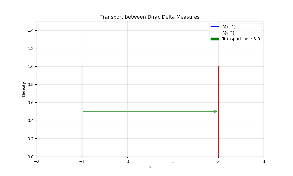
We can make this intuition more concrete. Consider the space of probability measures over the real line $\mathcal{P}(\mathbb{R})$. There is a natural embedding of the real line itself into $\mathcal{P}(\mathbb{R})$ where we map each point on the real line to the corresponding Dirac delta function located at that point:
\[f: \mathbb{R} \rightarrow \mathcal{P}(\mathbb{R}), \quad f(a) = \delta(x-a)\]One way to think about the Wasserstein-2 distance is that it’s the simplest metric on the space of probability measures $\mathcal{P}(\mathbb{R})$ for which this embedding is an isometry. This property makes the Wasserstein distance fundamentally different from statistical distance measures like the KL divergence, since the latter cannot handle distributions with disjoint supports.
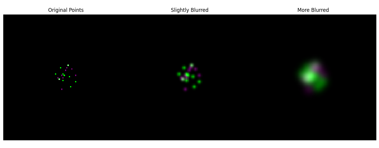
A “lift of the Euclidean metric” is not only a simple way to motivate the Wasserstein-2 distance, but it also helped me understand the motivations behind several research projects presented at the conference. For example, there was a talk given by Tudor Manole on co-localization in biology. Let’s say you have microscopy data for two populations of proteins, and you want to know how “correlated” the spatial locations of these proteins are in a cell. You do this by attaching fluorescent proteins to each type, such that one glows green under the microscope and the other glows purple. One way to measure the co-localization would be to compare the intensity of green and purple pixel-wise. However, this distance measure is problematic for several reasons, notably because it isn’t robust to differences in microscopes. Depending on the resolving power of the microscope, there can be more or less diffraction. You don’t want your measure of protein correlation to be highly sensitive to the measuring instrument. This is where optimal transport comes in. We know that the blurring process is “local”: given the noisy image, the true image will have the actual sources close in spatial distance. Optimal transport provides a distance measure where small perturbations in pixel intensity due to Gaussian noise correspond to small perturbations in the distance measure between the distributions.
“Wasserstein distance as the lift of the Euclidean distance” also helped me understand Yunan Yang’s work on stochastic inverse problems. Inverse problems are problems where given some observed effect, you try to deduce the cause. This covers a really broad array of problems, including many of the common problems that you see in physics. For example, if you want to know the mass distribution given gravitational field measurements, that would be an inverse problem. I also suspect that there is a connection to “parameter estimation” in statistics, as the term “inverse probability” is used in Bayesian statistics with roughly that connotation (though here I’m speculating).
A canonical example of an inverse problem is linear regression. With linear regression, we observe data $(X_i, Y_i)$ which we conjecture was generated by some linear model:
\[Y = \beta X + \epsilon\]We aim to estimate the parameters $\beta$. In ordinary least squares, this is done by minimizing the least squares cost function.
\[\hat{\beta} = \text{arg min}_\beta \|Y-X\beta\|^2\]Notice that this cost function is simply the Euclidean distance squared between the observed $Y$ and the model prediction $X \beta$. So we can re-express the above equation as:
\[\hat{\beta} = \text{arg min}_\beta \ d_E(X \beta, Y)\]In least-squares, we are trying to find optimal $\hat{\beta}$. But imagine that instead we generalize by trying to find the optimal distribution over $\beta$. This is where Wasserstein geometry comes in. Instead of minimizing a cost function involving the Euclidean distance (which leads to a point estimate), we minimize a cost function involving the Wasserstein distance (which leads to a distributional estimate). To make the connection more apparent, we can re-express the definition for Wasserstein distance in terms of random variables instead of in terms of couplings.
\[\begin{align} W^2_2(\mu, \nu) &= \inf_{\gamma \in \Gamma(\mu,\nu)} \int \|x - y\|^2 \, \gamma(dx, dy) \\ &= \inf_{\text{Law}(X) = \mu, \text{Law}(Y) = \nu} \mathbb{E}\|X - Y\|^2 \end{align}\]Normally, in optimal transport, we are given $\mu$ and $\nu$ and we want to find the transport plan that minimizes the cost between them. With stochastic inverse problems, we are given the final measure $\nu$ and the transport plan $T$ and we want to find the distribution $\mu$ (which I assume is usually constrained to fall into some variational class) such that the overall cost is minimized.
\[\hat{\rho}_\beta = \text{arg min}_{\rho_\beta} W^2_2(X_{\#}\rho_\beta, \rho_Y)\]This provides a bit of an abstract perspective on the data matrix $X$ in the context of least-squares: one can think of the data matrix as a kernel from parameters to output. This feels a bit abstract because it seems more natural to think of the parameters as defining a map from $X$ to $Y$ than to think of $X$ as defining a map from $\beta$ to $Y$. But there isn’t a real mathematical difference as both $X$ and $\beta$ can be viewed as linear operators whose co-domain is $\mathcal{Y}$: $X(\hat{\beta}) = \hat{\beta}(X) = \hat{Y}$.
(This notation is my own. I am not trying to replicate Yunan’s notation as trying to be perfectly faithful would increase the time it took to write this post with little apparent gain. It also helps to make the key point clearer to make the analogy with least-squares as obvious as possible.)
Regularized Optimal Transport
Another interesting throughline of the conference is regularizations of optimal transport. The most popular regularization of optimal transport is entropic optimal transport. It modifies the cost function to add a term proportional to the negative entropy of the coupling.
\[S_\epsilon(\mu, \nu) = \inf_{\gamma \in \Gamma(\mu, \nu)} \int \|x-y\|^2 d\gamma(x, y) - \epsilon H(\gamma)\](The regularization parameter $\epsilon$ has a straightforward physical interpretation as temperature $T$. This becomes especially apparent in “dynamical” formulations of entropic OT where we cast the problem in terms of learning the drift of a stochastic differential equation where the diffusion coefficient is proportional to the regularization parameter $\epsilon$. There also seems to be a suggestive analogy with the free energy $F = U - TS$, but I’ve given less thought to this perspective.)
To get an intuition for how entropic OT works, we can consider the problem of transporting the uniform distribution over the interval $[-L,L]$ to itself. Imagine that $\mu = \nu = \text{Law}(\mathcal{U}(-L,L))$. In unregularized OT (which corresponds to $\epsilon = 0$), we have that the transport plan is the identity map: as the source distribution and the target distribution are the same, the lowest cost transport plan is to not move anything at all. The optimal coupling is given as
\[\gamma(x,y) = \delta(y - x) \frac{1}{2L} \Theta(|x| < L)\](In general, with unregularized OT, if there exists a transport plan between the two distributions $\mu$ and $\nu$, then the unregularized coupling is given as $\gamma(x,y) = \delta(y - T(x)) \mu(x)$. This is a straightfoward consequence of the chain rule; $\delta(y - T(x))$ is precisely the conditional distribution $p(y|x)$.)
In unregularized OT, the support of our coupling is degenerate. The coupling is only supported on a one-dimensional submanifold of $\mathbb{R}^2$; equivalently, the conditional distributions $p(y|x)$ are only supported on a point.
With entropic OT, the optimal coupling will now have full support with respect to the product measure. If $(x,y)$ has positive density in the product measure $\mu \otimes \nu$, then $\gamma(x,y)$ will also have positive density (equivalently, we can say the Radon derivative $\frac{d\gamma}{d(\mu \otimes \nu)}$ is positive everwhere in $\text{Supp}(\mu \otimes \nu)$). A way to see this is to re-express the entropic OT cost function as a modified cost function with a term that is proportional to the log of the Radon derivative:
\[S_\epsilon(\mu, \nu) = \inf_{\gamma \in \Gamma(\mu, \nu)} \int \left[\|x - y\|^2 + \epsilon \log \left(\frac{d\gamma}{d(\mu \otimes \nu)}\right)\right] d\gamma(x, y)\]Heuristically, imagine we are solving for the optimal coupling iteratively and we have a test coupling $\bar{\gamma}$. If for any $(x,y) \in \text{Supp}(\mu \otimes \nu)$ we have that $\frac{d\gamma}{d(\mu \otimes \nu)} = 0$, then the modified cost function will be $- \infty$ at $(x,y)$ due to the log term. It will then be infinitely favorable to move some probability mass from some other location $(x’,y’)$ where the cost is finite. Furthermore, again heuristically, we would expect the conditional distribution $p(y|x)$ to be of a form such that the modified cost is independent of $y$. Otherwise, we could improve on the coupling by moving probability mass from a higher cost region to a lower cost region. (This argument is heuristic because it isn’t accounting for the fact that marginal constraints need to be obeyed.) It’s instructive to set the modified cost function at $y’ = x$ and $y = x$ equal to each other get an approximate functional form for the conditional probability density function:
\[\epsilon \log \left(\frac{d \gamma}{d (\mu \otimes \nu)}(x,x) \right) = \|x - y\|^2 + \epsilon \log \left(\frac{d \gamma}{d (\mu \otimes \nu)}(x, y)\right) \longrightarrow \frac{d \gamma}{d (\mu \otimes \nu)}(x, y) = \left(\frac{d \gamma}{d (\mu \otimes \nu)}(x, x) \right) e^{-\frac{\|x-y\|^2}{\epsilon}}\]This is all quite handwavey, but the key points I want to emphasize are that (1) the modified cost function naturally leads to Gaussianity in the conditional distributions, and (2) larger values of epsilon correspond to larger values for the covariance for the conditional.
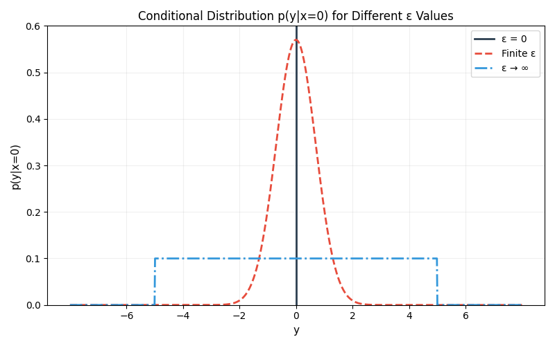
When $\epsilon = 0$, the conditional distribution is a Dirac delta. At finite $\epsilon$, there is some spread to our conditional distribution. And at $\epsilon = \infty$, our entropic OT solution becomes the product measure—the maximum entropy distribution with the marginals $\mu$ and $\nu$ (which is equivalent to the condition that the conditionals equal the marginal for all values of x: $p(y|x) = \nu(y)$).
If you’d like to learn more about entropic OT, I recommend these lecture notes by Marcel Nutz. He’s a Columbia professor who was also one of the hosts for the conference.
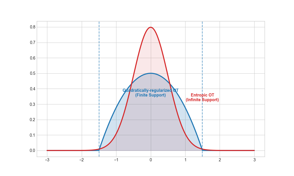
Even before attending the conference, I was already familiar with entropic OT. What was new to me was quadratically-regularized OT. With quadratically-regularized OT, we modify the unregularized cost function with the square of the Radon derivative of $\gamma$ with respect to the product measure, integrated over the product measure:
\[\mathcal{C}(\mu, \nu) = \int \|x-y\|^2 d\gamma(x, y) + \int \left| \frac{d\gamma}{d(\mu \otimes \nu)} \right|^2 d(\mu \otimes \nu)\]In many ways, entropic OT and quadratically-regularized OT are similar in that they both modify the unregularized OT cost function with a convex function of the Radon derivative of $\gamma$, integrated with respect to the product measure. If we let $R = \frac{d\gamma}{d(\mu \otimes \nu)}$ denote the Radon derivative, then in entropic OT our regularization term is $R \log R$, whereas with quadratically-regularized OT, our regularization term is $R^2$.
The key difference is that the quadratically-regularized cost function induces a sparse solution. If I can be honest, I’m not in love with the use of the term “sparse” in this context since it doesn’t quite accord with how I usually think of sparsity. But in any case, what we mean by “sparse” in this context is that the conditional distributions of the optimal coupling will not be fully supported on the codomain.
We can see where the sparsity comes from by again using the modified cost function framework that we used to analyze entropic OT:
\[\mathcal{C}(\mu, \nu) = \int \left[\|x-y\|^2 + \frac{d\gamma}{d(\mu \otimes \nu)} \right] \gamma(dx,dy)\]The Radon derivative is always non-negative, so we don’t have that vacuum effect that we had in entropic OT that made the coupling have full support. If we once again set the modified cost function at $y’ = x$ and $y’ = y$ to be equal to each other, then we have that:
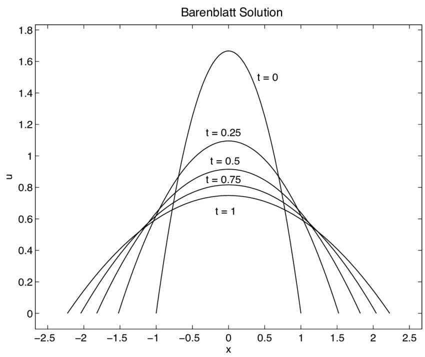
\[\frac{d\gamma}{d(\mu \otimes \nu)}(x, x) = \|x-y\|^2 + \frac{d\gamma}{d(\mu \otimes \nu)}(x, y) \longrightarrow \frac{d\gamma}{d(\mu \otimes \nu)}(x, y) = -\|x-y\|^2 + \frac{d\gamma}{d(\mu \otimes \nu)}(x, x)\]As the Radon derivative can’t be negative, what we actually have is a truncated parabola that terminates abruptly when the density reaches zero. Unlike a Gaussian, the parabola has finite width—this is where the sparsity of the conditional distributions comes from.
The talk that introduced quadratically-regularized OT discussed connections to Barenblatt’s equation and the porous medium equation. It felt like a bit of deja vu, as I had just finished Nigel Goldenfeld’s book on Statistical Physics about a month ago (It’s quite good! You should read it.) The book contained an extended, technical discussion of the Barenblatt equation in the context of renormalization group theory. I can’t comment on the connections the talk made between the two subjects as the discussion was too technical for me to follow.
There’s a fairly obvious analogy that entropic OT is to the KL divergence as quadratically-regularized OT is to the chi-squared divergence. I haven’t thought about the implications of this connection. (It doesn’t help that I’m not very familiar with the any of the more intrincate properties of the chi-squared divergence.)
Miscellaneous
There were lots of other interesting topics covered during the conference that I could talk about.
[Edit: The original version of this blog post gave the wrong definition of linearized OT. Sorry about that!]
I saw a couple different posters that involved linearized OT. With linearized OT, we approximate the OT distance by taking the $L_2$ norm of the difference between the transport map of our two measures, with respect to some reference measure.
In differential geometry, there is an object called the exponential map which takes elements of the tangent space and maps them to points in the manifold. (A visual analogy is that you can think of a person throwing a ball, like in a video game. The arrows emanating out of the person dictate a direction and a magnitude. If they then throw the ball, it will land somewhere. The function that relates the cartoon arrow emanating out from the person to the actual physical location in the world where the ball landed is the exponential map.)
Once you have the notion of an exponential map, it’s natural to define a logarithm map. Given a reference point $\sigma$, you can map points in the manifold to corresponding points in the tangent space of $\sigma$ by inverting the exponential map.
With linearized OT, you use the logarithm map associated with some reference measure $\sigma$ (often $\sigma$ will be something simple like the Gaussian) to map measures to the tangent space of $\sigma$. What exactly, mathematically, is the tangent space of a measure? It’s a space of functions which we can identify as transport maps. Let $T_\mu$ denote the transport map that pushforwards $\sigma$ into $\mu$. Given two measures $\mu$ and $\nu$, we can take the $L_2$ norm of the difference of their transport maps with respect to $\sigma$ to define the linearized OT distance.
\[\text{LOT}_\sigma(\mu, \nu) = \sqrt{\int \left|T_\mu - T_\nu \right|^2 d\sigma}\]The choice of reference measure matters because linearized OT is an approximation of the true OT distance between the distributions. The closer the reference measure is to the two distributions we are comparing, the better the approximation. (I was told by Sinho that the linearized OT distance is always an overestimate of the true OT distance, though I haven’t worked it out for myself yet so I don’t have a quick intuitive explanation for why that is the case.)
Sinho’s talk was quite interesting. It dealt with mean-field variational inference. “Mean field variational inference” corresponds to the variational approximation where we assume that, given a random vector $\vec{X} = (X_1, \ldots, X_d)$, the individual random variables are independent (or equivalently, we only consider measures that are product measures).
The way I think about variational methods is that they are a way of turning an infinite-dimensional, non-parametric problem into a finite-dimensional, parametric problem. You trade some accuracy for computational tractability. The hope is that if you choose your subclass correctly, the true non-variational solution will be close enough to the variational solution. Physics students are probably most familiar with variational methods from their quantum mechanics class when they have to approximate the energy of the ground state of a Hamiltonian by using an ansantz for the wavefunction. (Though as I typed out the above paragraph, I realized the space of product measures, while simpler in structure than the space of arbitrary measures, is still “infinite-dimensional”. So perhaps my story about variational approximations being about turning “non-parametric to parametric” problems isn’t quite right.)
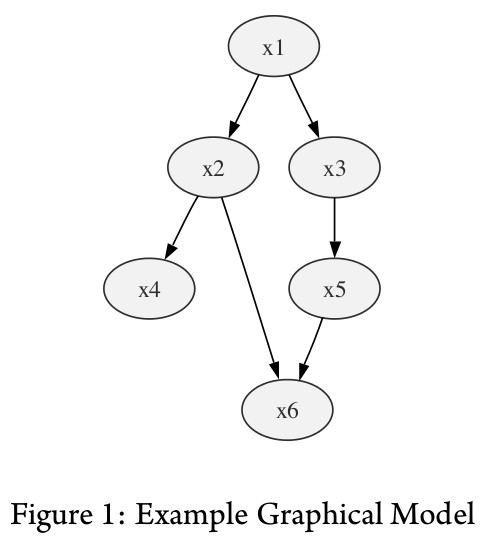
There was also a poster presented by collaborators on follow-up work. Mean-field theory is when you have a collection of random variables that are all treated as independent. But a natural way to relax the assumptions of mean field theory is with graphical models. Graphical models allow variables to have conditional dependency, but they control the nature of these conditional dependencies as represented by some underlying graph structure. Given a vertex (which is associated with a random variable), if you condition on all neighboring vertices, then the remaining variables become conditionally independent of the variable under consideration. You can also think of graphical models as generalizations of Markov chains, where the underlying graph structure in a Markov chain is linear (such that when you condition on any given variable $X_t$, variables after that time point will be conditionally independent of variables before that time point).
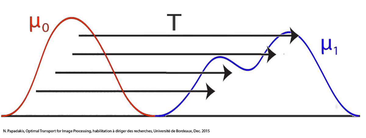
The last talk of the conference was given by Robert McCann. I had heard McCann’s name before due to McCann interpolation. Let $\mu$ and $\nu$ be two measures and let $T$ be the optimal transport map from $\mu$ to $\nu$. McCann interpolation says that the geodesic in Wasserstein space between any two measures can be found by linearly interpolating the transport map from the identity to $T$.
Mathematically, the McCann interpolation at time $t \in [0,1]$ is given by:
\[\mu_t = ((1-t)I + tT)_{\#} \mu\]where $I$ is the identity map and $\mu_t$ represents the measure at interpolation time $t$.
McCann gave a very technical talk on his recent work in microeconomics that I didn’t understand. It felt like good timing though as I recently finished the book “Econophysics” by Eugene Stanley, which gives an overview of some of the ways that physicists’ tools can shed light on financial data (it mostly covers the usual stuff these types of books cover like the Black-Scholes equation and the connection between stochastic differential equations and Brownian motion). Microeconomics has always been a sneaky passion of mine. For some reason, many of the topics I’ve been exploring in the past six months—statistical physics, stochastic differential equations—have made me want to revisit microeconomics, now with a stronger mathematical foundation.