Continuous Phase Transitions and the Dawn of Specialization

In my previous post “Phase Transitions As Global Optimization”, I explored a framework for understanding phase transitions through the lens of global optimization. In Landau theory, thermodynamic systems minimize their free energy by performing global optimization over the order parameter. In economics, firms maximize their profit by performing global optimization over the allocation of scarce resources. Despite the superficial differences, the unifying principle is that phase transitions correspond to non-analytic behavior in the argmin with respect to small changes in external conditions.

The example phase transition I used in the previous post was the classic case where a ferromagnetic system switches the sign of its magnetization as you change the sign of the external magnetic field. This can be neatly visualized using a magnetization versus free energy curve. If you plot how the free energy curve changes as a function of the external magnetic field, you can see how the location of the global minimum changes: for small positive $H$ field, the global minimum is at \(+M_0\). For small negative $H$ field, the global minimum is at \(-M_0\).

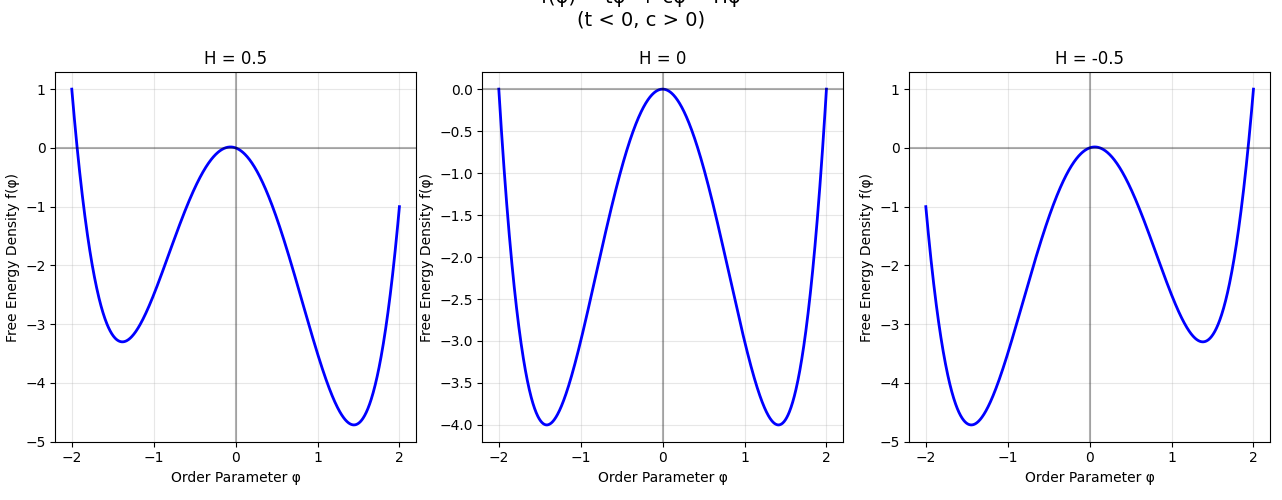
At $H=0$, there is a discontinuity in the magnetization—the argmin of the free energy. These are called first-order phase transitions. The nomenclature “first-order” is a bit obscure, but becomes clearer if you recall that all information about a thermodynamic system is captured by its partition function. The free energy is in fact proportional to the log of the partition function: $F = -\frac{1}{\beta} \log Z$. The magnetization $M$ is obtained by taking the derivative of the free energy with respect to $H$. The ferromagnetic phase transition is first-order because there is a discontinuity in $M$: a first derivative of the free energy.

But not all phase transitions will exhibit a discontinuity in the magnetization. There are also continuous phase transitions: phase transitions where the arg min of the order parameter changes in a non-analytic, but continuous manner. To get an intuition for how that could be possible, consider the graph below of this ramp function:

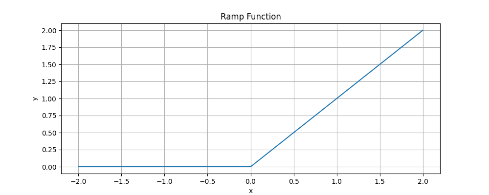
The ramp function is continuous everywhere, but is non-analytic at the origin. You can tell based on the kink at $x =0$. We can represent the ramp function as a piecewise function:

\[f(x) = \begin{cases} 0 & x \leq 0 \\ x & x > 0 \end{cases}\]

While the ramp function is continuous everywhere, there is a discontinuity in the first derivative at $x = 0$. We can generalize the ramp function by considering functions $f_n$ of the form:

\[f_n(x) = \begin{cases} 0 & x \leq 0 \\ \frac{x^n}{n!} & x > 0 \end{cases}\]

Each “generalized ramp function” $f_n$ is continuously differentiable up to its $(n-1)$-th derivative, before exhibiting a discontinuity at the $n$-th derivative. As $n$ increases, these functions appear increasingly smooth since we are pushing the discontinuity to higher-order derivative terms.

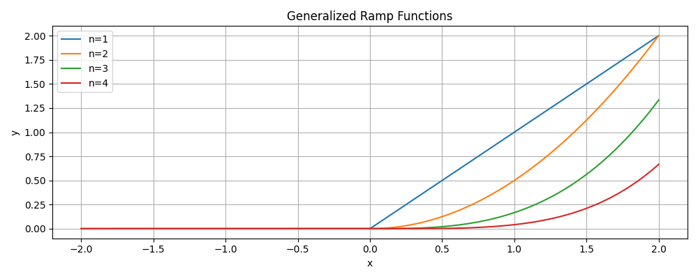
Just as generalized ramp functions become discontinuous at different orders, phase transitions can be classified based on the lowest derivative of the free energy that becomes discontinuous. This is called the Ehrenfest classification system. Since magnetization is the first derivative of free energy with respect to $H$, and we want the magnetization to be continuous at the phase transition, the simplest example of a continuous phase transition is a second-order phase transition.

The canonical example of a continuous phase transition is in the Ising model. When the number of spatial dimensions is greater than or equal to two ($d \geq 2$) and there is no external magnetic field, the system exhibits two phases. At high temperatures, the system is in the paramagnetic phase: disordered with no net magnetization. At low temperatures, the system is in the ferromagnetic phase: ordered with non-zero magnetization. At a critical temperature $T_c$, there is a phase transition. Above $T_c$, the magnetization is zero. Below $T_c$, the system continuously gains magnetization until at $T = 0$ (absolute zero), it reaches a magnetization of $\pm 1$, meaning all spins are either up or down.

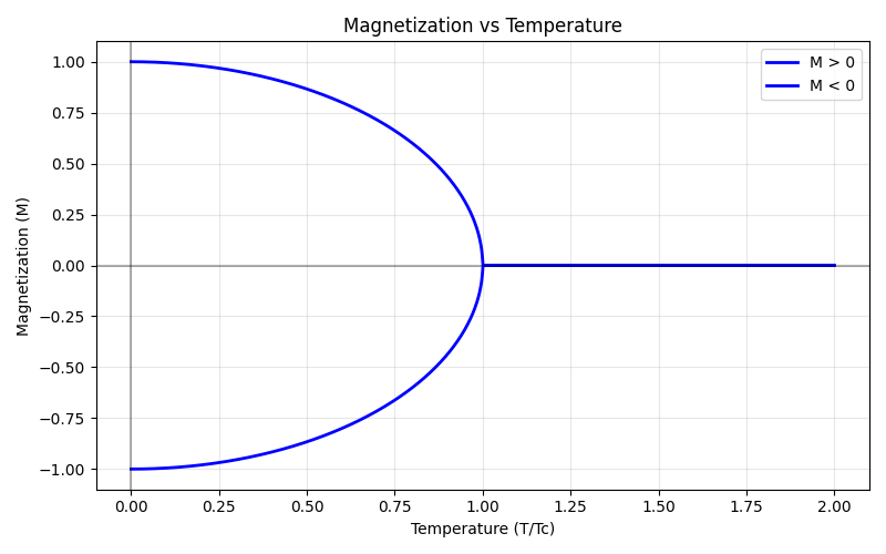
Like the first-order transition discussed above, we can visualize this continuous phase transition using a free energy versus order parameter curve. Here we have a simplified free energy with just two terms:

\[f(\phi) = t \phi^2 + c\phi^4\]

The quadratic term has a coefficient $t$, called the reduced temperature. It’s defined as:

\[t = \frac{T - T_c}{T_c}\]

The reduced temperature measures temperature relative to the critical temperature $T_c$ where the phase transition occurs. Rather than using absolute zero as our reference point, it uses $T_c$ as the zero-point. This makes it simple to identify the phase from the sign of $t$: when $t > 0$, we are in the disordered phase; when $t < 0$, we are in the ordered phase.

The graph below represents a continuous phase transition from disordered to ordered states. We can visualize the transition from paramagnetic to ferromagnetic phases by observing how the global minimum shifts as the reduced temperature passes through zero. For $t > 0$, there is one local minimum (which is the global minimum) at $\phi = 0$. For $t < 0$, there are now two local minima (which are both global minima) at non-zero values $\pm \phi_0$.

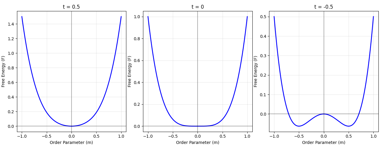
Here’s a visual picture: you should be imagining the free energy landscape as a rugged terrain with many valleys corresponding to local minima. As you change the thermodynamic parameters, these valleys both bob up and down in height and move through the space. A first-order phase transition occurs when one local minimum dips below the previous global minimum. This causes the system to instantaneously jump to the new global minimum—a discontinuity in the argmin.

But local minima don’t just bob up and down; they can also drift through the abstract optimization space. Sometimes, two local minima collide and merge into one; conversely, one local minimum can split into two. While first-order phase transitions correspond to jumps between minima, continuous phase transitions correspond to the merging and splitting of local minima.

We can revisit our economics metaphor. In that analogy, a first-order phase transition corresponds to switching between specializations (e.g., choosing between majoring in Math or English). Extending the analogy, a continuous phase transition corresponds to shifting from a generalist strategy to a specialized one. This makes intuitive sense: temperature measures disorder, with low temperature representing more ordered conditions. The more orderly the environment, the more it pays to specialize.

I don’t know much about history, but I have this image of the pre-modern world being one where people were self-sufficient in small family units. Each family had a piece of land and had to take care of all their needs. Life was difficult and unpredictable. If you didn’t repair your roof before the winter, the frostbite was gonna getcha. If you didn’t fortify your home regularly, the roving bandits from across the river were gonna getcha. And if you somehow survived both the frostbite and bandits, the semi-annual bout of syphilis was definitely gonna getcha. Nasty, brutish, short, etc.

In the pre-modern world, there was no room for specialization. Everyone had to be self-sufficient—able to farm, hunt, and defend themselves. But the modern world we live in is defined by specialization. How did this transition happen?

Here’s a minimal model. Imagine there are only two tasks: hunting and gathering. In primitive societies, everyone had to spend exactly 50% of their time hunting and exactly 50% of their time gathering.

But then slowly people started to specialize. It starts small: you’re behind on your harvest and won’t have enough barley stored for the coming winter. You’ve been talking with Joe next door and notice his farming expertise. Though you don’t completely trust him, you trust him enough to offer a trade: if he gives you his extra barley, you’ll go on an extra hunting trip. Joe accepts since you’re known as the best spear-thrower in town. You are now technically a specialist: you now spend 50.1 % of your time hunting and 49.9% of your time farming, as opposed to the previous fifty-fifty split. This is the dawn of specialization.

While there is a phase transition—people shift from generalists to specialists—this specialization is gradual. Eventually, these win-win trades create surplus, enabling more orderly societies and more complex economic arrangements. After millennia of this process, societies become so orderly and specialized that it’s unremarkable for someone to spend a decade of their prime working years studying statistical physics instead of pursuing a more honest living of hunting and gathering for one’s daily required calories.