Physics Meets ML

One of my favorite resources for learning more about work at the intersection of physics and machine learning is the website Physics Meets ML.

This website features work done by theoretical physicists with applications in machine learning. Though it hasn’t been updated in almost two years, it still has an interesting backlog going back to 2020. I am unfamiliar with even the basics of the vast majority of research that it shows, but I want to briefly highlight some of the work that I am more familiar with. I’ll present these in chronological order as listed on the website.

Neural Scaling Laws and GPT-3 - Jared Kaplan

Jared Kaplan is a theoretical physicist who used to work on cosmology and conformal field theory. But seeing the trends in AI, he switched to working on machine learning. He is a co-founder of the AI company Anthropic, best known for their signature LLM Claude.

This talk is about scaling laws. Scaling laws refer to how the performance of a neural network scales as you give it more inputs. It concerns the empirical relationship between four quantities:

• Data ($D$)
• Parameters ($P$)
• Compute ($C$)
• Loss ($L$)

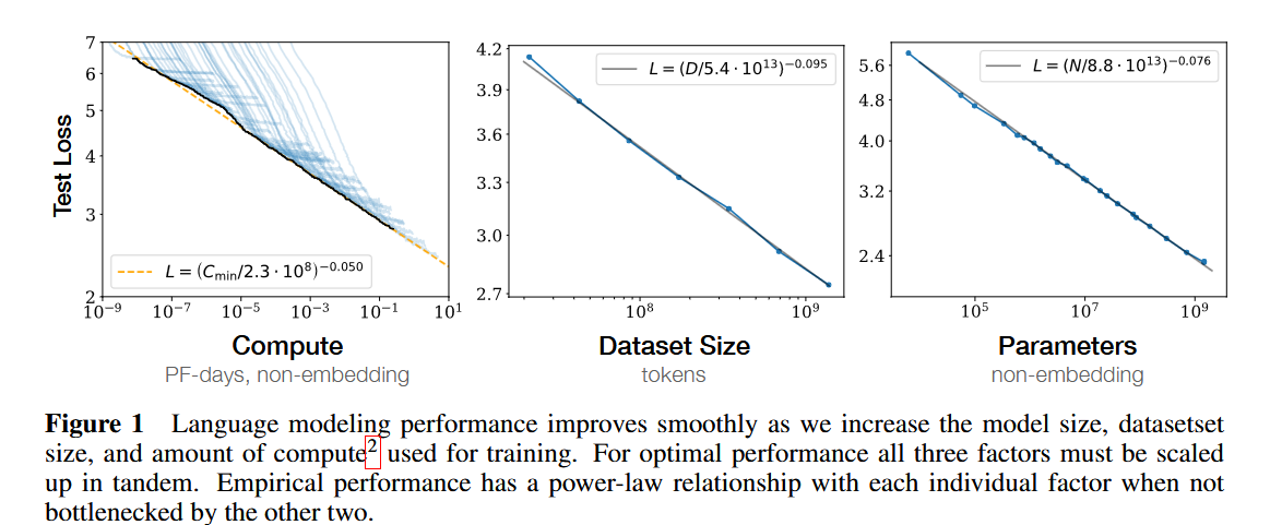
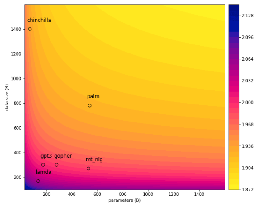
What was found is that if you plot e.g., compute versus loss on a graph, the empirical trend follows well-behaved mathematical curves. This was important for a couple of reasons. First, it allowed researchers to know how to more efficiently allocate resources. Using scaling laws, it was shown that LLMs would be more efficient if they had fewer parameters, but were trained on larger data sets. While I can’t find a source, I believe this insight was behind the improvement between GPT-3 and GPT-3.5. The original GPT-3, released in 2020, while powerful, wasn’t optimally trained given the neural network scaling laws.

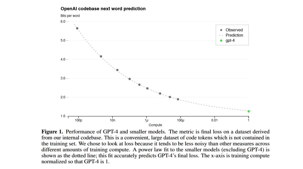
Second, as a consequence of scaling laws, you can predict given the amount of compute, what the loss will be. This was best demonstrated by OpenAI in their blockbuster announcement of GPT-4 where they showed a graph predicting GPT-4’s performance based on the best-fit curve generated by weaker LLMs.

Lastly, scaling laws implied that all you needed was to spend more on compute in order to have the LLMs improve. “The Scaling Hypothesis” was the big bet that OpenAI made that catapulted them to the forefront of AI development.

Feature Learning in the Infinite-Width Neural Networks - Greg Yang

I’m not familiar with this work, though I’ve been exposed to the idea of the infinite-width limit due to another entry that we will get to later on this list. But I watched Greg Yang’s interview on the Cartesian Cafe and was really impressed by both his story and the high-level summary he gave of his work. I will be taking a closer look at this.

There are many different meanings of the word “feature” in ML. But in this context, I believe feature means “a semantically meaningful aspect of the input”. The width of a neural network is the number of neurons in each layer.

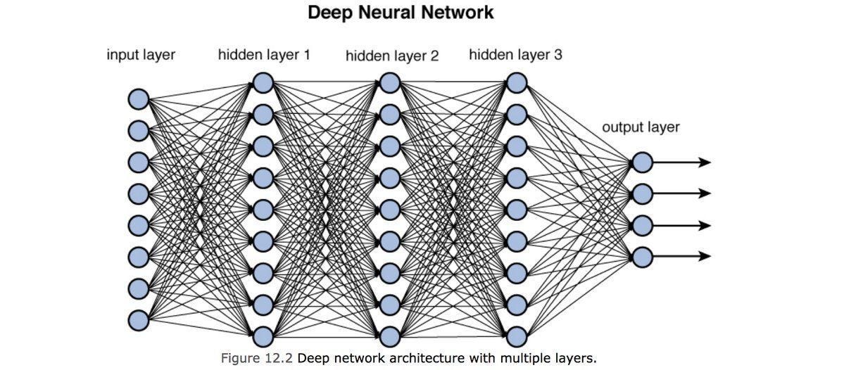
If I had to guess, the paper concerns the fact that when you have a finite-width neural network, it’s forced to learn semantically meaningful features. An example would be that if you have a finite-width digit classifier, it will be forced to learn about edges. But if you have an infinite-width network, it could just operate at the level of the pixel and still minimize the loss.

This is speculation on my part.

Explaining Neural Scaling Laws - Ethan Dyer

Again, not familiar with this specific work in depth, but I recognize Ethan Dyer’s name from past perusals of Google Scholar pages and arXiv abstracts. My subconscious associates him with good work being done.

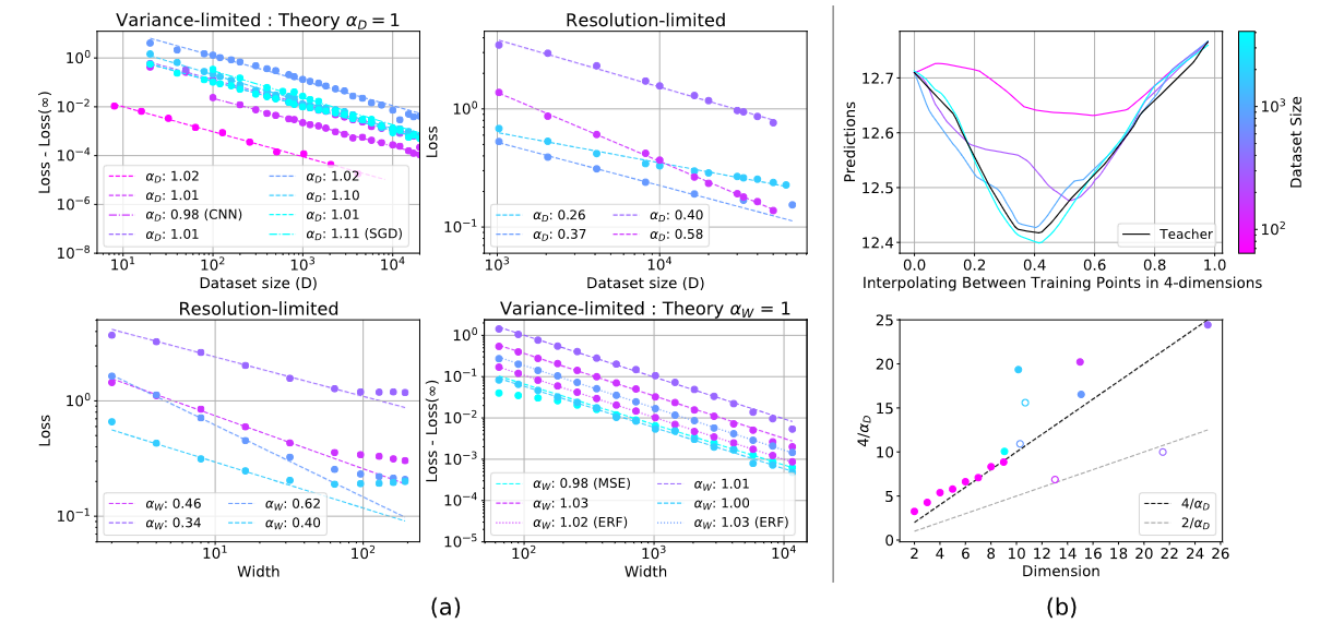
Interestingly, while the entry on Physics Meets ML is dated to 2021, there is actually a PNAS paper that goes by the same name that was published in 2024. If I had to guess, it’s the same project that took a while to get published somewhere, but this is just a guess. The paper claims to try to explain where the scaling laws come from. I don’t understand the terminology (“variance-limited” or “resolution-limited”), so I can’t really comment on what the paper is claiming. Might take a look at this, but the amount of new jargon that I would need to parse means this won’t be a priority for me.

Effective Theory of Neural Networks - Sho Yaida

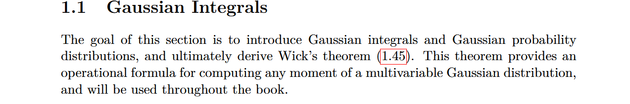
Sho Yaida and Dan Roberts released a book called ‘The Principles of Deep Learning’. The book’s goal is that while machine learning is an empirical subject, it’s much in need of theory. Both of them have theoretical physics backgrounds, and the book applies techniques from statistical field theory (e.g., perturbation theory from a Gaussian free theory) in order to analyze neural network behaviors in various limits. I’m like two chapters into the book, though I haven’t picked it up in a couple months (though I do plan on finishing it). It’s an interesting read, though I more so enjoy it for being a fresh, new way to revisit the fundamentals of QFT and statistical field theory (e.g., Wick’s theorem), than I enjoy it for making me view neural networks in a new light.

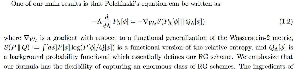
Renormalization Group Flow as Optimal Transport - Semon Rechnikov

If I had to guess, this was the talk that made me discover Physics Meets ML in the first place. I stumbled upon Jordan Cotler’s talk (the other co-author besides Semon on the paper) on YouTube during the doldrums of COVID and was instantly captivated. While it’s a technical paper, the main result is elegant: renormalization group flow can be viewed as Wasserstein gradient flow of field-theoretic relative entropy.

This paper is the most technical of the ones I’ve included, so it’s hard to summarize. But here’s an attempt at some intuition.

Consider the heat equation:

\[\frac{\partial u}{\partial t} = \nabla^2 u\]

While the calculus can look intimidating, the heat equation actually says something fairly simple: every point in space will “regress” to the average of its neighbors. If $u(x)$ is lower than its neighbors, then in the next time step it will go up. If $u(x)$ is greater than its neighbors, then it will go down. Over time, this results in the distribution becoming more flat and even as each point approaches the same height as its neighbors.

Now, what is the most flat distribution? The uniform distribution. And one property of the uniform distribution is that it’s the maximal differential entropy distribution defined on its support. This provides a perspective on the heat equation: while locally we can view it as a PDE, globally the distribution itself will be increasing its entropy over time. The entropy functional $S(u_t)$ is a monotone with respect to the dynamics defined by the heat equation. And if you choose the right metric on your space of measures, the heat equation is precisely what gives the direction of steepest descent with respect to the entropy functional—it defines a gradient flow.

The key insight of the paper is that renormalization group flow can be similarly formalized as a gradient flow in the space of measures over field configurations. The monotone in this case isn’t the differential entropy, but a specific relative entropy relative to a specific action $Q$ (which is related to the Gaussian free action).

On my to-do list for this blog is to give this paper a more proper treatment sometime in the future. I’m going to wait though, because in their follow-up paper “Renormalizing Diffusion Models,” the authors mentioned that a new paper “Score-Based EFT” is currently in the works. Hopefully that comes out sometime this year and I can review all three papers as a trilogy.