Thinking, Fast and Slow Time Scales

I didn’t get much from my two semesters of quantum field theory. But one idea that managed to make an impression on me is the concept of “effective theories”. An effective theory is a model that captures the important physics at a particular scale while ignoring details that don’t matter at that scale—like how you can describe the flow of water without tracking the individual water molecules. This perspective that different models of reality might be applicable at different scales wasn’t invented by quantum field theorists—at least I don’t think. It seems like a fairly old idea. But by way of the renormalization group, this understanding of how our physics changes as a function of scale is made precise, rather than simply remaining a philosophical idea.

I think that a simplified version of this idea can help us understand reaction networks, which are commonly used when modeling biological systems.

A reaction network is a way to represent the different states of a system and the probabilities of transitioning between these states. It’s represented by a weighted directed graph. The nodes of the graph represent the different possible states of the system. The edges are arrows, where the tail represents the starting state and the head represents the ending state. Associated with each directed edge is a weight $k$, which gives the strength of that reaction.

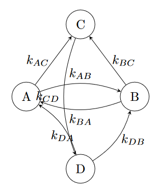
The reaction weights have units of inverse time. The higher the reaction rate $k$, the more likely the reaction is to occur. For example, given a reaction rate $k_{AB}$ which represents the rate of transitioning from state $A$ to state $B$, we have:

\[p_{AB} = k_{AB} \ dt\]

where $p_{AB}$ is the probability that, given the system is in state $A$ at time $t$, it will transition to state $B$ during the small time interval $dt$.

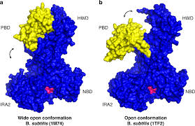
An example of a system that can be represented by a reaction network is protein conformation. Due to thermal motion and interactions with their environment, free-floating proteins transition between different shapes. If we want to understand how a protein’s shape evolves over time, we can represent it as a reaction network where each node is a conformation and each edge represents a transition between conformations.

What I’m going to show is that reaction networks in biology are best understood as defining effective theories. Implicit to every reaction network is two time scales: the slow time scale and the fast time scale. The slow time scale determines which transitions are considered to be possible. The fast time scale determines which states of the system are distinguishable from one another.

Thinking Slow

A wise man once said, “Anything is possible!” Given any two states $A$ and $B$, there is always some chance that the system could transition from $A$ to $B$ within a given window of time. To justify this statement, I could appeal to quantum mechanics (where the probabilities of transitioning between any two states can become arbitrarily small, but often don’t strictly vanish). But my contention is a bit more philosophical: the fully-specified reaction rate network is a complete graph—one where every vertex is connected to every other vertex.

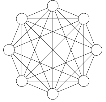
But in practice, the reaction networks we actually use are relatively sparse—where for any given state, transitions are only possible to some small subset of the remaining states. Where does this discrepancy come from?

While graphs represent relationships between discrete states, one can imagine the states of the system naturally living in some abstract continuous metric space. “Distance” in this space corresponds to how easily the system transitions between states: points that are close together should represent states that readily transition between each other, while distant points represent states that rarely transition.

(I will ignore the fact that the transition rates between states are often assymetric while distances are [by definition] symmetric. Trying to properly incorporate assymetric transitions would overly complicate the simple model that I’m trying to elucidate.)

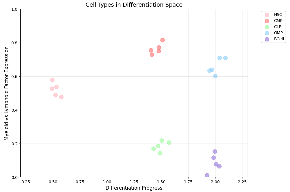
In the above graph, I represent the process of cell differentiation. During this process, a stem cell gradually determines its cellular fate (similar to how students choose different majors to develop specialized skills for different careers). Here, “HSC” stands for hematopoietic stem cells—stem cells that can differentiate into various blood cell types.

The graph represents cells’ progression in a 2D abstract space. The axes show differentiation progress (essentially time) and “myeloid versus lymphoid factor expression.” Myeloid cells are blood cells formed in bone marrow, like red and white blood cells, while lymphoid cells become immune system components like B cells and T cells.

While these axes have clear interpretations in this representation, that isn’t always the case in other visualizations. What’s most important is that proximity in the abstract space corresponds to likely cellular transitions.

A key insight emerges when we consider how systems actually move through this state space. For “nearby” states, transitions often look like random walks. For example, within a given cell type during differentiation, gene expression might fluctuate stochastically, causing small movements in this abstract space while maintaining the cell’s overall identity.

However, for “distant” states in our space, random walks aren’t sufficient—you need some form of drift. In our example, this drift is governed by the molecular processes driving differentiation.

In any system, there are two fundamental types of long-timescale transitions. The first type consists of gradual changes that necessarily unfold over long periods. The second type involves rare but discrete jumps between states—sudden, dramatic shifts that occur infrequently in the system’s state space.

Here’s a concrete example. Imagine our state space is the space of locations on Earth, and consider two points: Spain and America.

When Christopher Columbus first sailed to America from Spain, his voyage took roughly three months. While there were many stops and detours along the way, he was limited by ship travel—he could only cover so much distance each day. The process of going from Spain to America was necessarily gradual.

Now consider Carlos, a modern-day Spanish business consultant. Because of his work, he frequently travels to America where many of his clients live. He makes roughly four trips per year, though not evenly distributed: sometimes he’ll make back-to-back trips in the same month, other times he’ll go a whole year without traveling. But on average, he makes a trip every three months.

For both Christopher and Carlos, the timescale associated with transitioning from Spain to America is three months. But they represent opposite ends of the spectrum. For Christopher, the transition was gradual and continuous. For Carlos, the transitions are abrupt but infrequent.

Even though the distribution of these transitions are quite different, they are both long-timescale. If we wanted to model the behavior of Carlos or Christopher over the course of a single day, we would ignore the transitions associated with their voyages.

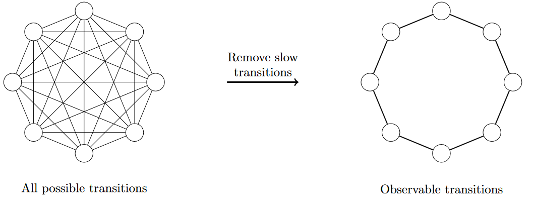
This is where sparsity in reaction graphs comes from: through the application of a slow timescale threshold. The procedure is simple: we define a minimum reaction rate $k_{\text{min}} \equiv T_{\text{slow}}^{-1}$ and delete every edge from the graph whose rate falls below this threshold (or equivalently, set those rates to 0).

In the case of cell differentiation, transitions between major cell types usually occur over the course of days. But if you are examining a cell over the course of an hour, then its cell type is unlikely to change. However, within a given cell state, there will still be fluctuations in RNA expression, protein levels, and other cellular characteristics. If we apply a slow timescale of an hour to our state system, then we end up with graphs like this one:

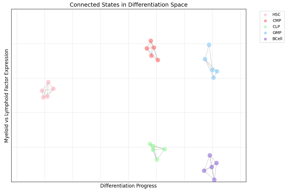
With the application of the slow timescale, our graph decomposes into separate components where each component corresponds to a cell type.

The slow timescale represents something like the “total observation time”—the length of time we are observing the experiment or natural process. When we apply a slow timescale threshold, we’re effectively saying “ignore any changes that are too slow to be noticeable during our observation period.”

(This is generally what we mean when we say something is “impossible”. It means that given some expected length of observing time, the probability of that event happening falls below a certain threshold.)

In the cell differentiation example, application of the slow timescale resulted in a disconnected graph. But you can imagine examples where the graph becomes sparse while still being connected. There is also a subtlety where when we talk about “transitions that are allowed to happen” we mean direct transitions.

Thinking Fast

Consider the time scales of the human body. There is the time scale of the thermal motion of hydrochloric acid molecules in the stomach. There the time scale of the subtle, pendulum-like swaying of limbs. There is the time scale of blinking, the time scale of circadian rhythms, the time scale of hormonal changes like puberty or menopause. There is the time scale of mortality.

And often, it’s not just that there exists a wide range of time scales, but there is a quasi-separation between them because transitions sharing a common mechanism tend to occur at similar rates. Going back to the human body example: the thermal motions of water molecules and hydrochloric acid are technically different due to their distinct chemical structures. But in the grand scheme of things—compared to the wide range of reactions that can occur in the body—they happen at similar time scales and both live in the “thermal motion” regime.

But when observing a system, there is often a shortest time scale below which we can’t resolve details. For example, if we want to track how someone’s emotions fluctuate throughout the day, we neither can nor need to measure the precise position and momentum of the hydrochloric acid molecules in their stomach.

When dealing with such fast time scales, we want our final graphical representation to exclude any rates $k$ larger than $k_{\text{max}} \equiv T_{\text{fast}}^{-1}$. However, we can’t simply delete edges corresponding to weights greater than $k_\text{max}$. So how do we proceed?

If applying a slow time scale corresponded to snipping edges, then applying a fast time scale corresponds to glueing nodes. When two nodes are connected by large reaction rates, the system quickly reaches an equilibrium distribution between them. The new node we create by gluing is a weighted average of the original nodes, with weights proportional to the fraction of time the system spends in each state.

This is similar to how a camera works: a camera’s exposure captures the average intensity of light over time. More generally, whenever we measure or interact with a system, there is always some finite duration of interaction—meaning we’re actually observing a time-averaged version of the system.

Consider this rectangular graph:

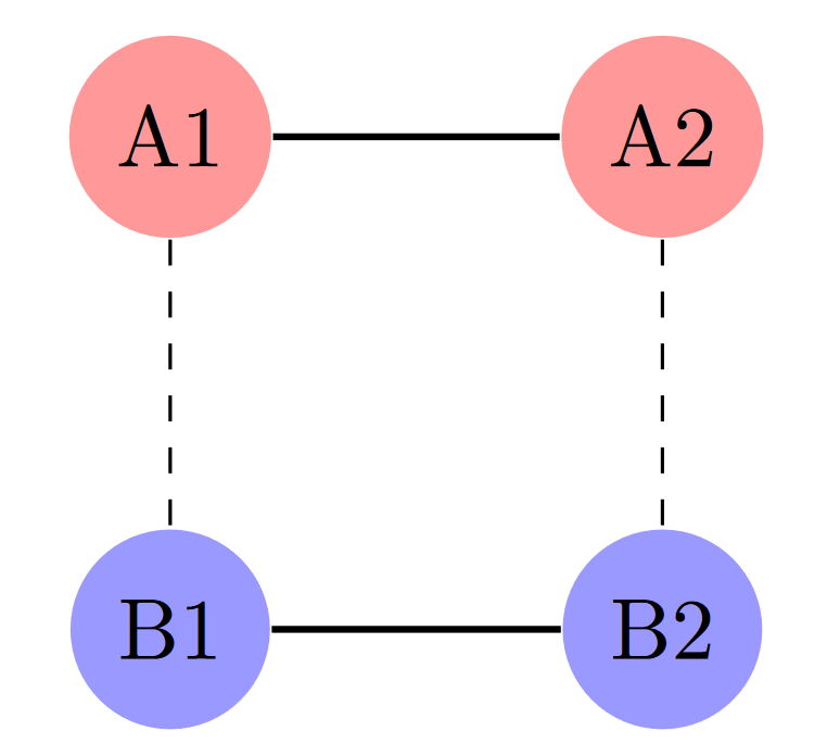
There are four states: A1, A2, B1, and B2. States sharing the same letter (A or B) are connected by large reaction rates, while states sharing the same number (1 or 2) are connected by smaller reaction rates. When we apply an appropriate fast time scale, the resulting graph combines the A states into one composite node and the B states into another.

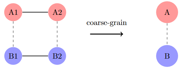
How do we find the weights for each component within a composite node? Throughout this post, I’ve shown reaction graphs as undirected to avoid visual clutter. However, reaction graphs are actually directed graphs, where the reaction rates $k_{AB}$ (A to B) and $k_{BA}$ (B to A) are distinct quantities. These rates determine the equilibrium distribution over nodes.

If $w_A$ represents the fraction of the composite node composed of state A, then:

\[w_A = \frac{k_{BA}}{k_{AB} + k_{BA}}\]

This formula makes intuitive sense: state A will be weighted more heavily when the reaction rate from B to A ($k_{BA}$) is larger, and vice versa for state B.

This explains what happens to nodes when we apply a fast time scale. But what about the edges? How do we determine the weight of the new composite edge? Just as each new node is a weighted average of its component nodes, each new edge weight is a weighted average of the component edge weights that formed it.

Let’s see this principle in action through a biological example. In biology, form implies function—what a molecule does is determined by its shape. This is often called the “lock-and-key” model. For example, enzymes latch onto specific sites on proteins, changing their shape and thus their properties. However, for an enzyme to successfully bind to its target site (called an allosteric site), it must be in the correct orientation.

To simplify this process, imagine the enzyme’s different orientations as points around a circle, where only the “right-facing” orientation allows binding to occur. We can represent this system with the following reaction network:

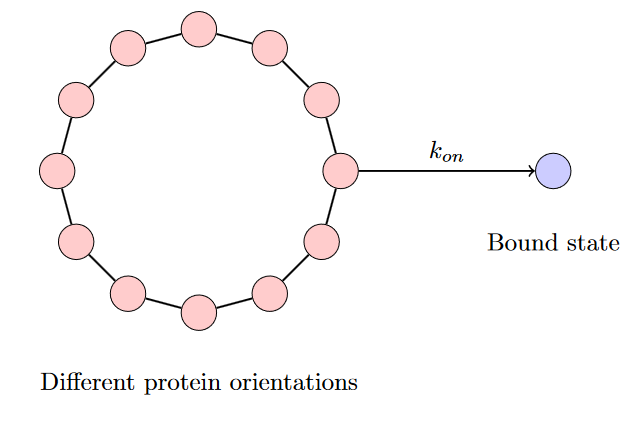
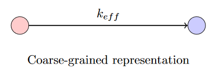
Notice that only when the enzyme is in the correct conformation is there an edge connecting it to the bound state. However, in practice, we cannot determine the exact $k_\text{on}$ rate for the correctly oriented enzyme—the thermal rotations of the protein are much too fast to measure. Instead, we work with an effective rate $k_{\text{eff}}$ that averages over all possible orientations:

\[k_\text{eff} = \int \frac{d\theta}{2 \pi} k_\text{on}(\theta)\]

This $k_\text{eff}$ is what experimental measurements actually report as $k_\text{on}$. This is quite revealing: a process can appear random at our level of description due to coarse-graining over microscopic details, even though the underlying dynamics are deterministic.

A Brief Note on Commutivity

So I’ve introduced two operations that can be performed on reaction network graphs: the application of a slow timescale where we prune edges whose reactions are too slow, and the application of a fast timescale where nodes connected by fast reactions are treated as composite nodes which represent equilibrium distributions over their constituent nodes.

But what happens if you want to apply both procedures to the same reaction network? Here, you have to be careful—you’ll get different results depending on the order.

To me, the correct order is clear: given a fast timescale and slow timescale, you should first apply the fast timescale, creating composite nodes, and only then apply the slow timescale where you prune edges.

Why would this be the correct order, conceptually? I’m not completely sure. One intuition is that when we prune edges, we are throwing away information; it’s a much more conspicuous, discontinuous operation than the more elegant approach of combining nodes as we do with fast timescales.