Bayes Theorem Is Just Chain Rule
I’m a bit embarrassed about how long it took me to notice that Bayes’ Theorem and the chain rule are actually the same thing. These are perhaps the two most fundamental equations in probability theory. Any derivation is likely to invoke one or both theorems as a step too obvious to even justify. I personally have used both of them countless times. And I didn’t notice that they were the same thing!
The chain rule in probability says that you can express a joint probability in terms of a conditional probability and a marginal probability:
\[P(A,B) = P(B|A) P(A)\]In English, this equation reads as “the probability that both $A$ and $B$ are true equals the probability that $A$ is true multiplied by the probability that $B$ is true given that $A$ is true.”
An important feature of the chain rule is that, given two propositions, there are two ways to decompose the joint distribution, depending on which proposition you choose as your marginal variable:
\[P(A,B) = P(A|B) P(B) = P(B|A) P(A)\]Since both decompositions equal the joint probability, we can set them equal to each other:
\[P(A|B) P(B) = P(B|A) P(A)\]If we then isolate $P(A|B)$ on one side, we get:
\[P(A|B) = \frac{P(B|A)}{P(B)} P(A)\]Which is precisely Bayes’ theorem!
The fact that Bayes’ theorem can be derived from the chain rule became relevant when I was learning about variational autoencoders. Before explaining the connection, let’s consider that for any two random variables $X$ and $Z$, there are five relevant probability distributions:
- The joint distribution $p(x,z)$: the probability that both $X=x$ and $Z=z$
- The conditional distribution $p(x|z)$: the probability that $X=x$ given that $Z=z$
- The conditional distribution $p(z|x)$: the probability that $Z=z$ given that $X=x$
- The marginal distribution $p(x)$: the univariate distribution of $X$
- The marginal distribution $p(z)$: the univariate distribution of $Z$
While there are five distributions, they don’t represent five degrees of freedom. These distributions are bound by certain relationships. The two chain rule equations remove two degrees of freedom. Initially, I mistakenly thought that Bayes’ theorem removed yet another degree of freedom. It was only after being briefly puzzled did I realize that Bayes’ theorem contains no new information beyond what’s already contained in the chain rule—because Bayes’ theorem is a direct consequence of combining the two chain rule equations together!
But what about the marginalization equations $\int p(x,z) dz = p(x)$ and $\int p(x,z) dx = p(z)$? Don’t these act as additional constraints? Indeed they do. The marginalization equations explain why, given just the joint distribution $p(x,z)$, we can derive all four other distributions. (More explicitly: given $p(x,z)$, we use the marginalization equations to get $p(x)$ and $p(z)$, then use the chain rule equations to get the conditional distributions $p(x|z)$ and $p(z|x)$).
However, in practice, integration is hard. Many sampling techniques and machine learning methods focus on modeling probability distributions without performing costly integrations. This challenge shows up in two common scenarios: calculating normalization constants (partition functions) in Gibbs measures like $Z = \int e^{-V(x)} dx$, and explicitly marginalizing joint distributions. This is why we often treat the marginalization equations as if they “don’t count.”
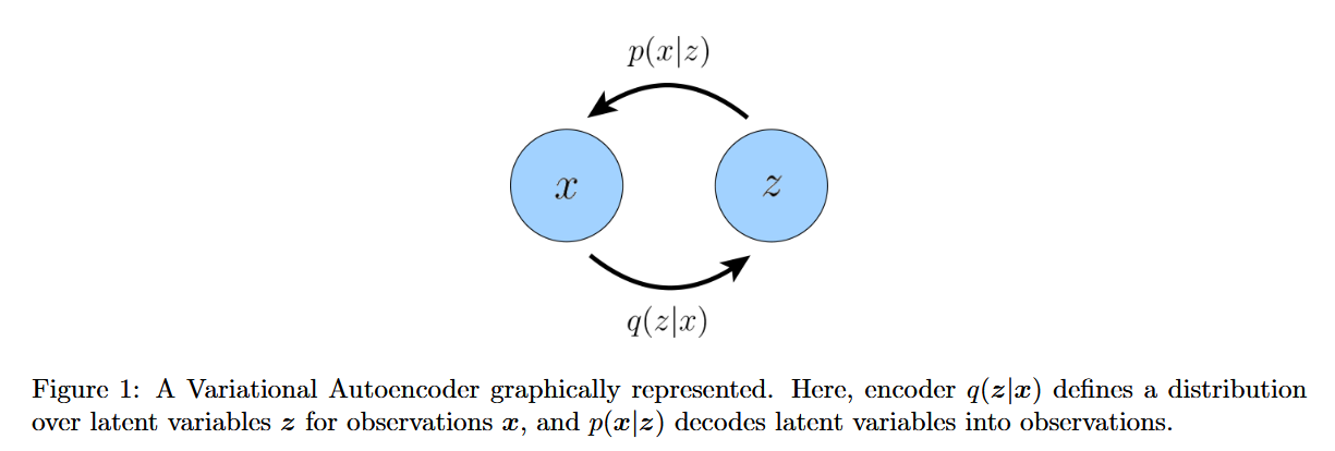
Ignoring the marginalization equations, we have three degrees of freedom. This becomes crucial in the context of variational autoencoders, which rely on specifying three distributions to determine the entire joint distribution:
-
$p(z)$: the “prior” distribution of your latent variable $Z$. (This terminology comes from the fact that when you encounter a data point $x$, your probability distribution over the latent variable updates according to Bayes’ theorem). This distribution isn’t learned, but is constrained to a regular distribution like a Gaussian.
-
$q(z|x)$: the encoder distribution which learns the mapping from data point $x$ to latent variable $z$ during training. (The distribution is denoted with “q” instead of “p” because we’re learning a variational approximation of the true conditional distribution $p(z|x)$—hence the name “variational autoencoder”).
-
$p(x|z)$: the decoder distribution which learns to generate data $x$ given the value of the latent variable $z$.

If there were only two degrees of freedom, the variational autoencoder architecture would be overdetermined and thus ill-posed. This also explains why you must constrain your prior (the distribution of the latent variable) beforehand. If you only tried to learn the encoder and decoder distributions, your system would be underspecified.